2 Probability Laws
2.1 Axioms of Probability
Given a sample space S, we will assign probability values to events (subsets)
which obey the following axioms:
-
P(A) >= 0 for every event A
-
P(S) = 1
-
If A1, A2,
are mutually exclusive events,
then
P(A1  A2
) =
P(A1) + (A2) +
(addition rule)
A2
) =
P(A1) + (A2) +
(addition rule)
Note: When we assign probabilities to all of the
subsets of a sample space, we create what is called a probability measure
on the space; behaves very similarly to area.
Can think of as Venn diagram, where total area is 1 (and so areas of subsets
are <= 1); then probability of subset is just its area.
ex:
of M & M's manufactured, 20% are red, 10% orange, 10% green, 10%
blue, 20% yellow and 30% brown. Thus if our experiment consists of
selecting one M & M at random and considering its color, our sample
space could be
S = {R, Or, G, Bl, Y, Br}
The logical assignment of probabilities to the single-element subsets of
the sample space is
P({R}) = .20
P({Or}) = .10
P({G}) = .10
P({Bl}) = .10
P({Y}) = .20
P({Br}) = .30
(we would usually write these as just P(R) = .20, without using
the set brackets, when we're dealing with single elements of the sample
space, even though strictly speaking probability values are associated
with subsets)
We would then get probabilities for other subsets by using the addition
rule!
So the probability of getting a red or a green M&M would be
P({R,G}) = P({R}) + P({G}) =
.20 + .10 = .30
Note: when a sample space is discrete, we usually assign
probabilities to individual elements, then find probabilities of other
subsets from these, as in the above example
Note: if the outcomes in our sample space are equally likely,
and there are N possible outcomes, then the probability of each outcome
is 1/N and thus the probability of any event A is
P(A) = n/N, where
n = number of outcomes for which A occurs
N = total number of outcomes
this is just the classical approach to assigning probabilities!
Some results about probabilities:
Theorem 2.1.2
P(A') = 1 - P(A)
proof:
Since AA' = S, P(AA')
= P(S) = 1
Since A A' =
A' =  ,
we can use the addition rule to get P(AA')
= P(A) + P(A')
,
we can use the addition rule to get P(AA')
= P(A) + P(A')
Thus P(A) + P(A') = 1 or
P(A') = 1 - P(A)
Theorem 2.1.1
P() = 0
proof:
= S',
so P()
= P(S') = 1 - P(S)
Note: sometimes much easier to find P(A') than P(A)!
From a Venn diagram, we can get an idea of how to find P(A1A2)
when A1 & A2 aren't disjoint:
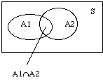
P(A1) + P(A2) counts the overlap twice, so subtract
P(A1A2)
This suggests the General Addition Rule:
P(A1A2 ) =
P(A1) + P(A2) - P(A1A2)
This can be used when events A1 and A2 aren't mutually exclusive
(disjoint), in which case the previous addition rule wouldn't apply.
ex:
ex:
On a particular football team, the probability that a player plays
offense is .60 and the probability that a player plays defense is .65.
Everybody plays one or the other. What's the probability a player selected
at random plays both?
Let A = the event a player plays offense, B
= the event a player plays defense
We want the probability of AB.
We can solve the general addition rule for P(AB)
to get
P(AB) = P(A)
+ P(B) - P(AB)
= .60 + .65 - 1
= .25
Note: Sometimes easiest to use a Venn diagram to compute probabilities;
just find the probability associated with each separate region.
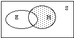
ex:
From the example above, what's the probability a child will have blonde
hair but not blue eyes?
With E and H as above, E' = the event a child doesn't have
blue eyes; then we want P(E'H).
The Venn diagram for the problem is shown, with all of the pertinent
regions labelled:
The shaded region is what we want; it's everything that's in H but not
in E. From the diagram, we can see that
P(E'H)
= P(H) - P(EH)
= .30 - .13
= .27
Previous section Next
section