3.4 Moment Generating Function
Recall: the moments of a random variable are useful to know, but not so
easy to find.
In cases where we know a formula for the p.d.f., can often find all
moments at once in a convenient way!
Def: Let X be a discrete random variable. Then the
moment generating function of X is the function of the variable t defined
as
mX(t) = E(etX)
-
the moment generating function is the expected value of the function
etX
-
the variable t is just a parameter (auxiliary variable), whose use will
become clear
-
the moments of X are hidden inside the function mX(t)!
ex:
AP example; recall that the p.d.f. for the score Z of a randomly selected
student was given by table
What's the moment generating function of the random variable Z?
Well,
mZ(t) = E(etZ) = 
= et (.15) + e2t (.20)
+ e3t (.40) + e4t (.15) +
e5t (.10)
Notice that this is a function of the variable t.
ex:
Flip a coin until you get a tail; let N = the number of flips. Then
we found previously that the p.d.f. was f (n) = (1/2)n.
Find the moment generating function.
As above,
mN(t) = E(etN) =
= 
= e1t * (1/2)1 +
e2t * (1/2)2 + e3t * (1/2)3
+ ...
= (et * 1/2)1 +
(et * 1/2)2 + (et * 1/2)3
+ ...
But this is another geometric sum, with first term a = et/2
and ratio r = et/2, whose value is thus
So
mN(t) = 
The above are functions of t; where are the moments of the random variables??
Theorem
If mX(t) is the m.g.f. of X, then the moments of X can be
found as
E(Xk) = 
i.e., to find the kth moment, take the kth derivative of the moment
generating function and evaluate at t = 0.
ex:
Example above; by the theorem,
E(N) =  =
=  (by the quotient rule)
=  =
=  = 2.
= 2.
This is the mean of N.
From this we can find the variance of N:
var(N) = E(N2) - E(N)2
= 6 - 22 = 2.
Why do we care so much about finding moments?
-
gives easy way to compute mean & variance
-
can identify the type of a random variable by looking at its moment generating
function, as stated by the following:
Theorem If two random variables have the same moment generating
function, then they have the same p.d.f .
This will be useful to us in the future, when we're trying to determine
what type of random variable we get when we look at specific combinations
of other random variables!
Properties of moment generating functions
Let X be a random variable, mX(t) its moment generating
function, and let c be a constant. Then the moment generating functions
of certain modifications of X are related to the moment generating function
of X as follows:
-
the moment generating function of the random variable cX is
mcX(t) = mX(ct)
-
the moment generating function of the random variable X + c
is
mX+c(t) = ect mX(t)
-
Let X1 and X2 be independent random variables
with moment generating functions
mX1(t) and mX2(t). Then the
moment generating function of the random variable X1 + X2 is
mX1+X2(t) = mX1(t) * mX2(t)
These results will be of use to us later. The proofs of these follow from
the properties of expectation discussed earlier.
The Geometric Distribution
Def: A random variable X is a geometric random variable if
it arises as the result of the following type of process:
-
have an infinite series of trials; on each trial, result is it is either
success (s) or failure (f). (Such a trial is called a Bernoulli experiment.)
-
the trials are independent, and the probability of success is same on each
trial. (The probability of success in each trial will be denoted
p, and the probability of failure will be denoted q;
thus q = 1 - p.)
-
X represents the number of trials until the first success.
(In short, a random variable is geometric if it "counts the number of trials
until the first success.")
ex:
Consider the "flip a coin until you get a tail" experiment above; then
N (= # of flips until a tail occurs) is a geometric random variable, with
p = 1/2: N counts the number of trials until the first success.
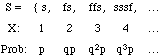
The sample space of such a process can be written as below; the value of
the random variable X associated with each possible outcome is shown beneath;
and the probability of each outcome is given beneath that. (The probabilities
just come from the multiplication rule for independent events.)
Thus the probability density function of a geometric random variable
X with probability of success p is:
f(x) = pqx-1 = p (1 - p)x-1,
x = 1, 2, 3, ...
Its moment generating function can be shown to be
mX(t) = 
(using a technique identical to that used in the "flip a coin until a tail
appears" example above).
We can thus use the moment generating function to find the moments,
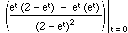
and hence the mean and variance and standard deviation:
E(X) =  =
=  (from the quotient rule)
=  = 1/p (using the fact that
p = 1 - q )
= 1/p (using the fact that
p = 1 - q )
E(X2) =  =
= 
=  =
= 
var(X) = E(X2) - E(X)2
= q/p2
So the mean and variance are
m = 1/p
var(X) = q/p2
(so the standard deviation is s
=  )
)
ex:
Dice game; pick a number from 1 to 6, then keep rolling until get that
value. Let X = total number of rolls needed to achieve this. Then X is
a geometric random variable: it counts the number of trials until the first
success.
The probability of success on each trial is here p = 1/6. Thus
from the above, the expected number of rolls until the desired number appears
is E(X) = 1/p = 1/(1/6) = 6.
(This is pretty much what we would have anticipated!) The variance is
var(X) = q/p2 = (5/6)/(1/6)2 =
30, so the standard deviation is s
= 5.48 , which indicates that the value of X will usually fall in
the range 6 +- 5.48; thus we should not be surprised if the number of rolls
needed to get our number is as few as 1 or as many as 12.
ex:
Consider the Pennsylvania daily number lottery, discussed before, in
which the probability of winning on any given day is 1/1000. Now let N
be the number of times you play before winning the first time. Then N is
a geometric random variable, since it's counting the number of trials until
the first success, with p = 1/1000. Thus the expected number
of plays is E(N) = 1/p = 1/(1/1000)
= 1000; thus you should expect to have to play 1000 times before
winning! Since you would then be down $1000 (since it costs $1 to play),
and would only recoup $500 for winning, this isn't such a great situation.
Notice that this agrees with our previous results, in which we determined
that, on average, you should expect to lose $.50 each time you play.
Cumulative probability function
The cumulative probability function F(x) of a geometric
random variable X with probability of success p
is
F(x) = 1 - qx = 1
- (1 - p)x
(This follows by summing the values of the p.d.f., and using the
formula for the value of a finite geometric sum.)
ex:
For the lottery example above, what's the probability that you'll win
in a year (312 days, not counting Sundays) or less?
Want P(N <= 312) = F(312) = 1
- (1 - .001)312 = 1 -
.999312 = 1 - .732
= .268;
thus there's only about a 1 in 4 chance that you'll win in a year if
you play every day!
Previous section Next
section