4.2 Expectation, Variance, Moments, Moment Generating
Function
Consider: in discrete case, the expected value of a random
variable X is defined as
i.e., it gives the weighted average of all possible values of X
-
cant quite do this in continuous case, since P(X=x) = 0 for
every x!
-
still, want E(X) = weighted average of all possible x values
Try instead: approximate the continuous distribution by
a discrete one, as follows:
Suppose possible values for X lie within some interval [a,b].
-
break the range of possible values into n subintervals of equal width;
let the points of subdivision be
a = x0, x1, x2, ... , xn
= b; the width of each subinterval will be Dx
= 
-
from the definition of the density function, the probability that X lies
between xi and xi+1 = area under density curve
from xi to xi+1, i.e.,
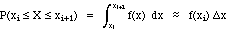
as long as Dx is small.
-
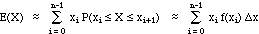
approximate X by a discrete random variable which takes on the values x0,
x1, ... , xn-1 - i.e., if the value
of X lies between xi to xi+1, round it down to xi
. Then the expected value for this "discretized" approximation to
X is given by the sum of the products of the x values and the probabilities
from above:
-
get a closer approximation to X by using more closely spaced points; should
get "true" value for the expected value of X in the limit as the number
of subintervals approaches infinity; and thus should have
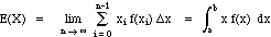
by the definition of the definite integral.
We use the above to motivate the definition of the expected value of a
continuous random variable (extending it to the case wgere the possible
values lie in the infinite range from - to
):
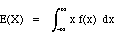
Def: If X is a continuous random variable, then its
expected value is defined as
-
as before, we also call this the mean of X, denoted m
ex:
Let X be the weight of cereal in a randomly selected box, as in the
example from the previous section, and suppose it has the density function
Then the expected value of X is
=  (note that f(x) = 0 for x < 14 and x > 15)
=  =
=  = 14.33
Note that the value of the mean is less than the midpoint of the interval
[14, 15] of possible values; this follows because the density function
is higher on the left end of the interval, indicating that X is more likely
to lie close to 14 than close to 15.
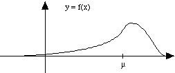
In general, E(X) gives the balance point of the density function:
if the region between the density curve and the x-axis were cut out of
a piece of wood, the location of the mean would be the point on which the
piece would balance.
For any function H(X) of X, we define the expected value of H as
Thus the moments are
The variance is
We have the same properties for expectation as before:
-
E(cX) = c E(X)
-
E(X+Y) = E (X) + E (Y)
As before, these give an alternate formula for computing the variance:
ex:
For the above "cereal density",
So
var(X) = E(X2) - E(X)2 =
205.5 - (14.33)2 = .0565
s = .24
Note: the standard deviation measures the expected deviation
from the mean, as before; thus it measures the spread of the density function,
i.e., how widely spread the values tend to fall from the location of the
mean.
The moment generating function is again defined as
and is used as before to find the values of the moments by differentiation:
Previous section Next
section