When investing for retirement, it’s typical to make contributions to a retirement account on a regular and frequent basis – maybe monthly or bi-weekly, through witholding from each paycheck. This is not just convenient, but helps to average out market-timing risk. If you put in a lump sum once a year (as some employers do with their contributions), and the market happens to be on an upswing that day, you may be inadvertently buying high and overpaying, whereas if the market is down you might be unintentionally getting a bargain. If you had some sense of where the market was headed, you could wait until the market was at a low point before making your investment, but market timing is well known as a way to lose money in the long run – we’re not very good at determining where the market’s going in the short run . By putting in regular frequent contributions, you can average out some of the risk – you’ll sometimes be buying high and sometimes low, but the ups and downs will generally balance out over the year. You’d have to be very unlucky to hit daily market troughs with all 12 or 24 or 26 contributions, whereas you only have to be unlucky once to hit a trough with a lump sum. This technique is commonly known as “dollar cost averaging” for its tendency to average out the cost of the investments you’re buying.
What’s Good for the Goose…
If it makes sense to use dollar-cost averaging with contributions while investing, why wouldn’t the same hold true for withdrawals during retirement? If you take a single annual lump-sum withdrawal at the beginning of the year to provide for that year’s spending, you may be withdrawing at a market trough and thus “selling low”. Just as with investing, it makes sense to distribute the withdrawals throughout the year, taking them monthly or even bi-weekly, to average out the market ups and downs. Of course, this involves some extra work in selling from accounts multiple times during the year, but this can be automated with some mutual fund accounts. And it has the advantage of making retirement funding look a lot like the working years – you get a regular “paycheck” from your accounts, which can help to guide spending throughout the year. The annual amount needed can be determined by applying some suitable withdrawal scheme, as discussed here and here, and then divided into 12 or more equal parts for withdrawal during the year.
There’s another advantage as well. By taking a lump sum out at the beginning of the year, you’re removing a large chunk of your investments from the market, which means it loses the growth opportunity for the remainder of the year. In down years this might be a good thing – you’ll have essentially (inadvertently) sold high, before the decline in portfolio value. However, since the market on average grows (by about 6.8% annually for the S&P 500 from 1871 to the present with dividend reinvestment and after adjusting for inflation), you’ll more often miss out on growth than avoid a loss. Given compounding, the difference can be significant over the years.
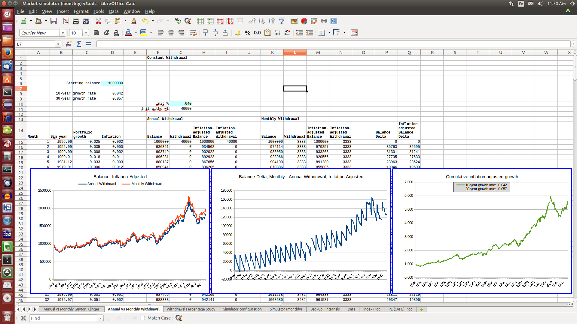
The screenshots below show results from several simulation runs using a spreadsheet-based simulation calculator to create simulated economic scenarios using market data from 1900 to the present, based on Robert Schiller’s freely available and widely used data set. The simulations use a constant inflation-adjusted withdrawal scheme, comparing annual with monthly withdrawal. The portfolio starts at $1,000,000, and the withdrawal rate is $40,000 per year, inflation adjusted, corresponding to the well-known “4% rule”. While there are lots of reasons why such a constant-withdrawal scheme isn’t the best scheme to use in practice, it illustrates most straightforwardly the difference between an annual and a monthly withdrawal regimen; other schemes show similar behavior. The sawtooth chart displays the monthly difference in portfolio balance between the monthly and yearly withdrawal schemes. The sawtooth shape results from the large lump-sum annual withdrawal depleting the balance of the annual-withdrawal scheme at the beginning of the year, while the balance of the monthly-withdrawal scheme gets reduced gradually, month by month.
The two example scenarios show that the difference in balance grows over the course of the retirement period, with the monthly withdrawal scheme being ahead almost always, and quite significantly under good market conditions. This is what we expect, using the reasoning above. For the scenario below corresponding to bad market conditions, in which there’s actually a negative annualized inflation-adjusted return over the first decade, there are times when the monthly-withdrawal scheme portfolio balance is below the annual-withdrawal scheme balance (as expected for true negative growth), but it still exceeds it in the long term even with the low overall growth. In this case both the annual and monthly withdrawal schemes run out of funds before the end of the desired retirement period, which is why it makes sense to consider an adaptive withdrawal scheme rather than a constant scheme, as discussed in other articles on this website on the Guyton-Klinger scheme and techniques for evaluating different withdrawal schemes. But the monthly withdrawal scheme still provides a little more than one additional year’s worth of withdrawal at the end due to the higher overall balance. Indeed, the only scenario in which the monthly scheme would perform more poorly than the annual scheme in the long run is if there’s overall negative growth throughout the retirement period, which is (thankfully) a pretty remote possibility, and disastrous overall.

We can get a statistical sense of the advantage of the monthly withdrawal approach by running repeated simulation scenarios and computing the average difference in balance over the retirement period for all the simulations. As expected, this shows that on average the monthly withdrawal scheme leaves us with a higher portfolio balance than the annual scheme. The smooth upward rise in the balance-difference graph below just reflects the average dividend-reinvested inflation-adjusted growth rate of the market over the period from 1900 to the present (the interval used to select simulation data), which is about 6.3%.

Conclusion
The above simulation data reinforces what we might reasonably expect – that dollar cost averaging of withdrawals during retirement, by taking monthly (or more frequent) withdrawals from our portfolio, helps to reduce market risk and provide additional growth on average when compared with the lump-sum single-annual-withdrawal approach.
Caveat
This information is presented as-is, with no guarantee as to accuracy or freedom from errors. This document and associated spreadsheet is intended as an observation for informational purposes only, and should not be used in retirement planning without cross-checking and correlating with other sources of information and consultation with a certified financial planner. I’m an enthusiast, not a professional, and being human I make mistakes. Your retirement funding is far too important to rely significantly on any unvalidated information!
Spreadsheet Download
- Spreadsheet used to generate statistics and graphs (OpenOffice/LibreOffice format)
The spreadsheet is open-source software licensed under the Gnu General Public License v2. This gives you the right to use the spreadsheet for your purposes, and adapt it (create a derived work) as you see fit as long as you make the new spreadsheet available for other users. See the link above for license details.
Data source for economic data
U.S. Stock Markets 1871-Present and CAPE Ratio, Robert Schiller, Yale University Department of Economics.
Articles in this series
-
Life Tables and Retirement Planning
-
Retirement Withdrawal Strategies: Guyton-Klinger as a Happy Medium
-
Variable Withdrawal Schemes: Guyton-Klinger, Dynamic Spending, and CAPE-Based
-
Comparing Retirement Withdrawal Schemes: Efficiency, Deficiency, and Disruptiveness
-
Retirement Withdrawal Efficiency Revisited: Variable Lifespan and Annuities
-
Annual or Monthly Withdrawal? Dollar Cost Averaging in Retirement
-
Over-valued, Under-valued, or Just About Right? Assessing Retirement Portfolios in Current Conditions