One of the most important decisions in retirement is the withdrawal strategy from a portfolio. This determines both our quality of life (how much we have to spend each year) and how likely our funds will last over the course of our retirement. One natural issue is that we don’t know how long we’ll live, so don’t know what the duration of our retirement will be. Though there are some reasonable ways to estimate what period we should plan for (as discussed in another article on this website), we can never be completely sure that we won’t live longer than we’ve planned, which should be a good thing, but isn’t if we run out of money. And the market conditions throughout the course of our retirement are similarly unknown, and this can make a huge difference between success (having all the funds we need throughout retirement) and failure (running out of money). Thus we need some strategy to adapt for this uncertainty.

The withdrawal scheme is a key tool to help adjust for market-related changes in our portfolio and the uncertainty of the retirement timespan. The withdrawal scheme is the formula/algorithm/system we use to determine how much to take out of our portfolio each year for spending. There are a number of popular approaches, several of which will be discussed here. They have different properties which affect our lifestyle (how much we have to spend) and our success probability (whether we’ll outlive our assets).

The Constant Withdrawal Scheme

The first and most basic scheme is inflation-adjusted constant withdrawal. In this scheme you take out the same amount every year, with an adjustment for inflation. Thus if you have a $1000,000 portfolio, you might decide to take out the equivalent of $35,000 each year. You’d take out $35,000 the first year; then for the second year, you’d see what the inflation rate was over the first year (from government statistics or the like), and add this on for the second year’s withdrawal. For example, if the inflation rate was 2.3%, you’d add on $805 (2.3% of $35,000), and take out $35,805 for the second year’s spending. You then repeat this process each year to get that year’s withdrawal from the withdrawal of the year before.

This scheme is very simple to implement, and has the very nice feature that your spending level and thus lifestyle will be the same from year to year – after all, you have the same amount each year after adjusting for inflation, so have the same buying power. In fact, this is the basis for the well-known “4% Rule”, which advocates this approach using 4% of your initial portfolio as your initial withdrawal – in our case, this would be $40,000, adjusted for inflation each year after.

But one significant gap with this method is that it takes no account of the remaining portfolio value when deciding each year’s withdrawal – it looks just at the previous year’s withdrawal and the inflation rate. When market conditions are weak for an extended period of time, especially in the early years of retirement, the portfolio can be drained quickly, causing us to run out of funds. Taking a withdrawal without considering the available balance is a very unnatural thing to do in any case – none of us would blithely take out $40,000 from a portfolio of $100,000 at age 70 and expect the portfolio to last over our retirement. There’s also the opposite (much better) problem, which is that if, due to booming market conditions, our portfolio blossoms and we end up with some multiple of our initial holdings, this method has us take out the same inflation-adjusted amount when we could potentially be enjoying a much better lifestyle. Again, this is unnatural – most of us would be thinking twice if we were taking just $20,000 annually from a portfolio of $3000,000.

As an aside, it’s worth noting that the “4% Rule” was developed from observations in the 1990’s, and reflects growth rates and lifespans that may no longer be applicable. Many financial planners are suggesting a lower initial rate like 3.5% (as used in the example) or less to reduce the chance that you will outlive your funds. See the article from the New York Times in the references for a discussion.

The Constant-Percentage Scheme

Another popular scheme is the constant-percentage scheme. In this scheme, a fixed percentage is selected as the amount to withdraw from the portfolio each year. Thus in our previous example, if a retiree selects 3.5% as the percentage to withdraw from the portfolio annually, with an initial portfolio of $1000,000, then he’ll take out $35,000 the first year, as before. However, for the second year, the amount taken out depends on the portfolio value at that point, which depends on the market. Suppose the market booms (a la 2013), and his portfolio at the beginning of the second year has grown to $1,300,000. Then the withdrawal for that year will be 3.5% of $1,300,000, or $45,500. Time to party! On the other hand, if the market tanked over the course of the year (shades of 2008), and his portfolio value at the beginning of the second year is only $650,000, then his withdrawal will be 3.5% of $650,000, or just $22,750. That’s some serious belt-tightening to endure from one year to the next.

The above illustrates one of the biggest disadvantages of the constant-percentage withdrawal scheme – the amount withdrawn exactly tracks the markets, and as we’ve seen they can be pretty volatile year to year. Having much of the portfolio in less-volatile holdings like bonds can reduce the volatility, but not eliminate it completely, and might also expose the retiree to risk from having portfolio growth that’s too slow to keep up with inflation in the long run. This scheme doesn’t take inflation into account in any case – you’re looking just at the portfolio value, not whether it has or has not kept pace with inflation.

But one key advantage of the constant-percentage withdrawal scheme is that you’re guaranteed not to completely deplete the portfolio – since you’re only taking out a percentage of the portfolio, you’ll never be left with nothing. Of course, with a withdrawal rate that’s too high, the portfolio can get small enough that it’s effectively nothing from the perspective of funding your retirement, so it’s important to select a reasonable rate. And under consistently bad market conditions the portfolio can similarly shrink, but this would generally occur under market conditions so bad that other schemes would be bankrupted anyway.

Guyton-Klinger: A Happy Medium

The two schemes discussed above can be distinguished by their focus on maintaining either the portfolio or the annual withdrawal. The constant-percentage scheme can be viewed as a scheme that looks only at protecting your portfolio without concern for your lifestyle, while the constant-withdrawal scheme looks only at maintaining your lifestyle without looking at the portfolio. The constant-withdrawal scheme is purely focused on the present, while the constant-percentage scheme is mostly focused on the future.

In reality, we’re all both focused on our year-to-year lifestyle as well as portfolio preservation. We’re not going to blithely deplete our portfolio with mindless withdrawals, nor are we likely to shrug off huge annual dips in our income. A reasonable compromise might be to do something like the following: start out with a constant-withdrawal approach, but if the amount being withdrawn gets too out of whack with the portfolio value (either too high for a shrinking portfolio or too low for a blossoming one), then make an adjustment – force a pay cut on ourselves or give ourselves a raise. That’s exactly the gist of the Guyton-Klinger scheme, developed by Jonathan Guyton and William Klinger.

In this scheme, we select an initial withdrawal rate, say 4%. We then select “guardrails” around this percentage to indicate when to take action. If our annual inflation-adjusted withdrawal, as a percentage of our portfolio, is above the upper guardrail, i.e., we think it’s too high a percentage of the remaining portfolio, we impose a pay cut. If the annual withdrawal is below the lower guardrail, indicating that our portfolio has grown enough that we’re taking out too small a percentage, we give ourselves a raise. The “spread” of the guardrails and the size of the pay cut or raise are the parameters for the model. Typical values might be to set the guard rails 20% above and below the base withdrawal rate, so at 4.8% and 3.2% for our example above, and to use a 5% pay cut and raise to adjust if we go outside those bounds.

This approach can help address the problems with both of the simpler constant-withdrawal and constant-percentage methods. It tries to help us maintain our lifestyle by only imposing a change if we edge outside the established bounds, and in that event limits the change to only the amount we’ve selected as the pay cut or raise. In the example above, we’d maintain constant spending power (inflation-adjusted) until we found that a particular year’s withdrawal would exceed 4.8% of the remaining portfolio value, and at that point cut our spending by only 5%, leaving us with 95% of last year’s spending power. Most of us can adjust fairly readily to living off 95% of our accustomed income.

Similarly, it keeps a close eye on our portfolio to make sure it doesn’t get depleted too quickly (by looking at the upper guard rail), or grow large without us being able to enjoy our additional wealth (by giving us a raise when we hit the lower guard rail). It’s thus a nice medium between the simplistic constant-withdrawal and constant-percentage schemes.

Aside

In fact, each of the simple schemes can be considered as a special (limiting) case of the Guyton-Klinger method. If we set the guard rails very wide – 0% for the lower rail and 100% for the upper – then the scheme will never hit them, and we’ll just take out the inflation-adjusted constant withdrawal every year, which is just the constant-withdrawal strategy. If we set the guard rails very close to the target value, then we’ll do a withdrawal adjustment almost every year which will push us back to the target rate, yielding essentially the constant-percentage scheme. We’ll see this graphically below when we do some investigatory simulations. (Note that the constant-percentage scheme isn’t exactly a special case of the simple Guyton-Klinger scheme described above – with a fixed amount for pay raise or cut, we will tend to overshoot a bit the target rate, so won’t exactly mirror the withdrawals we would take via the constant-percentage scheme. To completely duplicate the constant-percentage scheme we’d have to adjust the Guyton-Klinger scheme to allow variable cuts and raises based on the distance from the target rate. While lots of variations on the scheme are possible, we won’t discuss these here.)

It’s also worth noting that the Guyton-Klinger scheme involves an additional adjustment beyond the guardrail-driven withdrawal adjustment above (the “Modified Withdrawal Rule”, where the withdrawal isn’t adjusted for inflation in certain market conditions); see the Article “Using Decision Rules to Create Retirement Withdrawal Profiles” listed in the references for a complete description.

A Career in Modeling

It’s useful to be able to compare these schemes more formally, especially under different market conditions. In simple cases the results are easy to anticipate. Under a rising market, the constant-percentage scheme will give us annual pay increases as our portfolio grows, as will the Guyton-Klinger scheme (eventually, based on hitting the guard rail). The constant-withdrawal scheme will give us the same inflation-adjusted amount year after year, while allowing our portfolio to grow significantly. Under a falling market, our annual withdrawals will decrease annually under constant-percentage and Guyton-Klinger, causing a dent in our lifestyle but protecting the portfolio, while the constant-withdrawal scheme will potentially drain our assets, leaving us destitute.

But the market rarely just rises or falls – it’s up and down with business cycles and annual fluctuations. How does each scheme respond under varying conditions? In particular, how would each scheme have fared over historical scenarios taken from past market performance? And how would they fare over simulated random scenarios where the market behaves in some sense similarly to how it has in the past?

Fortunately, there are a number of tools that can help in this regard. One very useful tool is cFIREsim, a web-based portfolio withdrawal analysis tool that allows you to see how a portfolio would behave over historical market scenarios going back to 1871. It has many options, including asset allocation and accounting for additional income from Social Security and the like, and provides a number of different withdrawal methods for exploration, including Guyton-Klinger. Another similar very useful tool is FIRECalc, a predecessor to cFIREsim, but this includes only some more basic withdrawal schemes, and in particular doesn’t have Guyton-Klinger.

For our explorations here we’ll be using a spreadsheet-based simulation that provides full flexibility in adjusting the parameters for the withdrawal schemes and allows for creating specific graphs for investigating the relative performance of the schemes. The spreadsheet uses market information similar to that used in cFIREsim and FIRECalc (see the references), and provides facilities for constructing either historical simulations from 1928 to the present or synthetic simulations based on the historical market data arranged into random sequences. (See below for some justification on the rationale for and reasonableness of this approach.)

The things we’ll be looking at are the things a retiree would care about:

• Annual withdrawal, both absolute and as a percentage of portfolio
• Portfolio balance and its dependence on the market conditions

Withdrawal Scheme Comparison

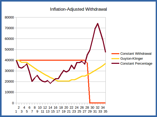
The graphs embedded in the images below show the performance of the three schemes discussed above over a couple of different historical scenarios: the 35 year periods beginning in 1969 and 1978. In each case the starting portfolio is assumed to be $1000,000, and the portfolio is assumed to be allocated as 75% stocks invested in the S&P500, 20% treasury bonds, and 5% treasury bills. This looks at how each withdrawal scheme would have performed in good and bad market conditions over the course of a 35-year retirement period.

Note that the values for the annual withdrawal and portfolio balance have all been adjusted for inflation – that is, they are all given in “starting year dollar values”. In this way we can directly compare withdrawals and balances, eliminating the effect of inflation. Note that with this adjustment the constant-withdrawal scheme withdrawals will all be constant, at the initial value; the graph will thus be a horizontal line, as seen in the charts below, and can serve as an easy reference for the other schemes to see if times are hard or life is good regarding our annual allocation.

Bad Market Conditions – Retiring in 1969

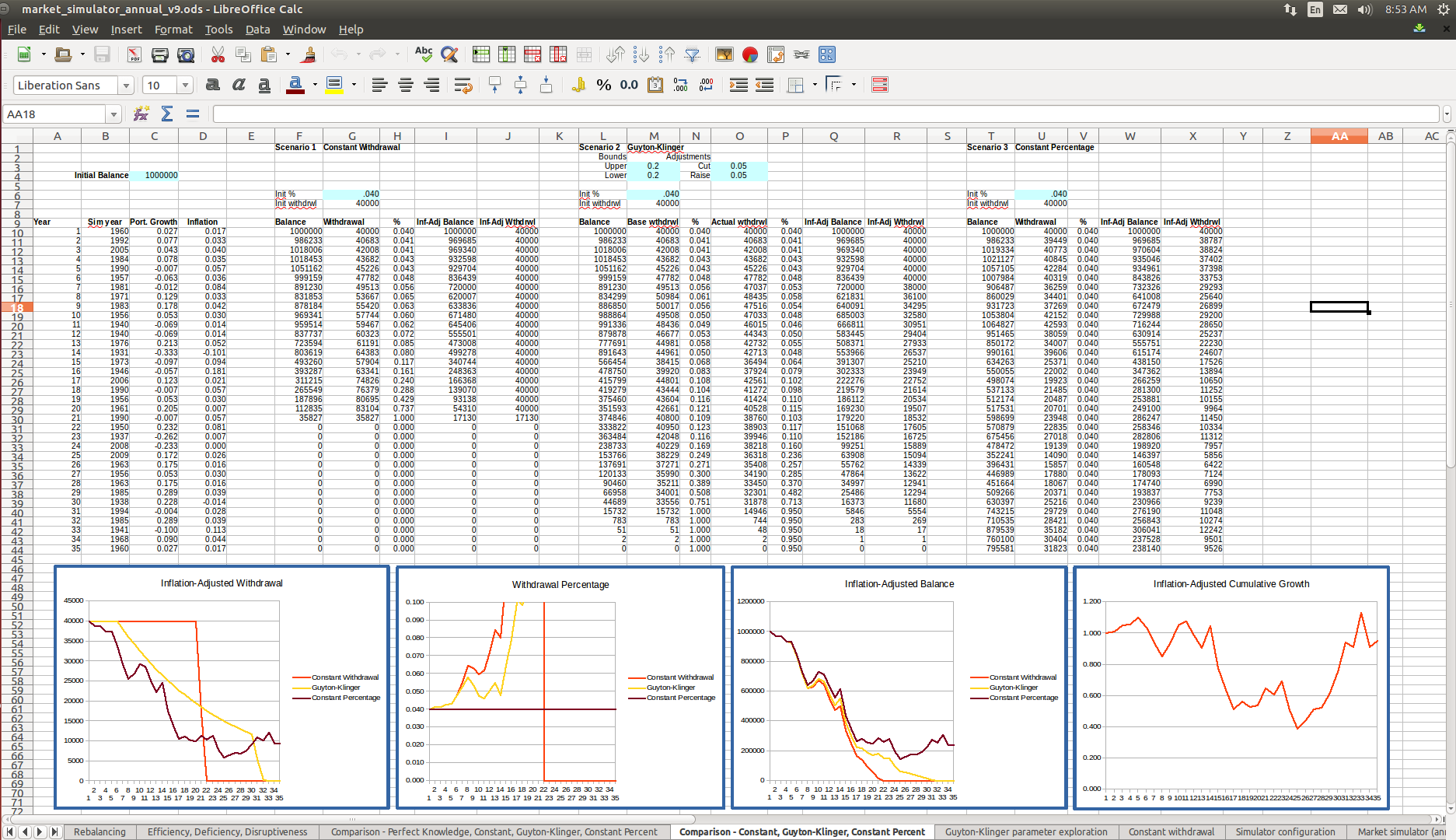
The first scenario is the historical scenario that has us retiring in 1969. In this case we have to endure the horrible market conditions of the 1970’s as our first decade in retirement. As seen in the graphs in the screenshot above from the market simulator, if we do a simple constant-withdrawal scheme, we rapidly deplete the portfolio during this decade of high inflation, and even though we then have the 80’s and 90’s with their good market conditions, the portfolio is too depleted to ever recover, and we run out of funds before the end of the desired 35-year period.

The constant-percentage scheme keeps us from critically depleting the portfolio during this first decade, which allows it to recover nicely in the following years, but it imposes some sudden and severe drops in income in years 5 and 6 that would be painful to endure. The withdrawals are restored when the market recovers, and even has us withdrawing much more than initially in the last years when the market is booming and portfolio is large. But the changes are again sudden, making this scheme put us in a position of sudden feast-to-famine and then famine-to-feast.

The Guyton-Klinger scheme is similar to the constant-percentage scheme in imposing some pay cuts to make sure the portfolio isn’t irrecoverably damaged during the bad market years, but it does this more slowly, decreasing our income by just 5% per year, although over multiple years. It similarly restores our income when the portfolio recovers, but again at a slow and steady rate. And the portfolio tracks the constant-percentage portfolio fairly closely, recovering when the market has recovered.

Good Market Conditions – Retiring in 1978

In good market conditions like those illustrated in the screenshot above, all the schemes are successful in the sense that we are never at risk of running out of funds. However, the constant-percentage and Guyton-Klinger schemes boost our spending power as the portfolio grows, whereas the constant-withdrawal scheme just plods along as our assets skyrocket. But again, the constant-percentage scheme has our income gyrating wildly during the tech bubble in the late 90’s, growing quickly and then falling just as quickly. The Guyton Klinger scheme smooths out the bubble – we benefit (more slowly) from the boom, but are buffeted from the bust.

This brings up a central question: what makes for a “good” retirement market condition versus a “bad” market condition? The key is in the graph of the cumulative net market growth, seen in the screenshots above. This is the cumulative growth of the portfolio, adjusted for inflation. A “bad” market condition is one in which this graph hovers around 1 for many years, indicating no real growth after inflation. This means we’re taking funds out of our portfolio, and the market isn’t doing anything to replenish them. A “good” market is one in which this graph steadily grows, indicating that there’s real growth adding to the portfolio.

The especially crucial period is the years right after retirement – the first decade, say. If there’s little real growth during this period, we risk depleting the portfolio to an extent that there’s too little for it to recover even if good years follow. That’s what happens in the 1969 scenario above – the 70’s are so bad that even the boom markets of the 80’s and 90’s can’t help the portfolio recover once it’s reduced over the first decade. On the other hand, if the first decade is good – and we don’t get greedy and take out more than we’ve planned – then the portfolio will have been able to grow and will be robust enough to weather subsequent bad market conditions without risking depletion. That’s what is illustrated in the 1978 scenario – the growth in the portfolio over the 80’s and 90’s makes it such that we can weather the bursting of the tech and housing bubbles.

Observations and Conclusions

Experimenting with retirement portfolio withdrawal schemes and seeing how they fare over various historical and simulated market conditions can help to select one that addresses our main concerns, especially running our funds dry prematurely. Having a scheme that adjusts for the variability in the remaining portfolio balance due to market fluctuations would seem to be key for most investors. The Guyton-Klinger scheme is one such scheme that provides the additional benefit of smoothing our annual withdrawals from the radical ups and downs that sometimes occur in the market.

However, it’s important to note that the Guyton-Klinger scheme isn’t perfect – it’s quite possible to have especially bad market scenarios in which even this approach exhausts the portfolio prematurely, or leaves us with so little that it’s effectively gone (see the screenshot below of an especially bad simulated scenario). The key to our portfolio successfully funding us through our desired retirement period is for the market to be able to replenish our withdrawals through growth; if there’s no growth, or even negative growth, this won’t be possible. Even putting your money in cash and withdrawing 4% per year for 25 years doesn’t guarantee stability, because even though you won’t be subject to risk from falling markets, you still risk having your spending power severely eroded by inflation. Even annuities provide an imperfect solution – though they’re designed as insurance against your annual withdrawal running dry, they may not provide protection against inflation, or if so provide a meager return that greatly constrains your lifestyle. So there’s unfortunately no real panacea; a certified financial planner can help to work out the best arrangement for your circumstances and temperament.

The Early Years are Key

Just as in investing for retirement, the early years are key when starting retirement. When investing, it’s the compounding of contributions from early in your retirement savings that make a huge difference in your portfolio size at retirement. When retiring, it’s the early years of retirement – say, the first decade – that greatly determine whether your funds will last and support you throughout your retirement. Unfortunately, it’s the market environment over this period that determines if the portfolio will be able to recover from your withdrawals or will be depleted by them. That’s something you can’t predict, though there are some mitigations. You can put portfolio funds in more conservative investments (bonds, say) that have a less volatile profile, and so will be less likely to significantly negatively affect the portfolio during this early period. But by the same token they’ll also provide more limited growth opportunity, which means you would be forced to have a lower initial rate of withdrawal.

You could also consult market barometers to see if your portfolio at retirement is “over-valued” or “under-valued”, as discussed in another article on this website. If the market has been in a significant period of growth, and indicators like the S&P500 price-to-earnings ratio are significantly higher than the long-term average, you might conclude that your current balance is somewhat over-valued from a long-term perspective, i.e., likely to be corrected downward over the next decade or so. In this case you might want to be more conservative in your (initial) withdrawal rate – maybe using a 3.5% or 3.3% rate rather than the traditional 4% rate. Similarly, if the market has been in a bear market for some time, you might feel your portfolio is under-valued and is likely to grow in the near future, and thus target a somewhat higher initial withdrawal rate. But of course, any such prediction of what might happen in the future is uncertain at best, and really deserves consultation with financial experts who spend every day looking at issues like this.

Next Steps

The above considers various withdrawal schemes qualitatively, looking at their performance under various market conditions. While we can see that some perform better than others under certain conditions, especially regarding failure (running out of assets), it doesn’t give a sense of how two schemes compare when their failure probabilities are roughly the same. This leads to the question of how we might compare schemes beyond looking at failure rates, and particularly whether there’s any quantitative measures we can use to perform such a comparison. This is considered in the next article in this series, Perfect Knowledge in Retirement Planning: Efficiency, Deficiency, and Disruptiveness.

Spreadsheets and Simulators

Several spreadsheets and simulators that can be used to explore the Guyton-Klinger and other withdrawal schemes are available for download at the bottom of this page.

Guyton-Klinger Personal Worksheet and Market Simulator

Personal Worksheet

This download includes a personal worksheet for calculating and tracking withdrawals using the Guyton-Klinger withdrawal scheme. This spreadsheet is designed to compute the recommended withdrawal each year over a series of years using this algorithm. It requires that parameters be selected for the algorithm – the initial withdrawal percentage, the percentage guardrails, and the pay-raise/pay-cut percentages – and for portfolio balances and inflation rates to be provided each year so the recommended withdrawals can be computed. This spreadsheet is designed to be used over time –  each year a new row will be populated on the spreadsheet, using your portfolio balance for that year. This is thus a long-term personal worksheet, based on your actual balances and economic conditions as they evolve over the years.

The spreadsheet comes pre-populated with some example values for a hypothetical retirement that started in the year 2010 with an initial portfolio balance of $1000,000. A user would change the blue cells in the spreadsheet to correspond to his/her retirement year and portfolio balance, and the relevant inflation rates for the retirement years.

Guyton-Klinger Market Simulator

The download also includes a market simulator designed to be used to investigate the effect of using different parameter values within the Guyton-Klinger withdrawal algorithm for different simulated market conditions. The spreadsheet compares the Guyton-Klinger withdrawal scheme for 6 sets of parameters, with different guardrails and pay raises/cuts. It assumes an initial portfolio value of $1000,000, and uses simulated market conditions to see how annual withdrawals and remaining portfolio balance vary over the course of a 30-year retirement for each of the 6 schemes. Each time the spreadsheet is refreshed, a new simulation is run with new randomly-selected market conditions. Graphs show the (inflation-adjusted) annual withdrawal each scheme provides, the percentage of the portfolio this withdrawal represents, and the remaining portfolio balance.

General Market Simulator

This is a more general market simulator that investigates a number of different withdrawal schemes, including Guyton-Klinger, and constant percentage, among others. It is a more advanced tool than the above Guyton-Klinger simulator.

For both simulators, the market condition simulations are drawn from the historical returns for stocks, bonds and inflation from 1928 through 2014. The simulator by default selects a random set of years from this set, and applies the corresponding stock/bond/inflation values. Thus each simulation represents a hypothetical scenario where the market conditions are as given by the randomly selected sequence of years. The simulator can also be configured to use a straight historical sequence with a randomly selected start year. This will then show how each of the 6 schemes would have performed over the selected historical 30-year period.

Spreadsheet Simulator Use

The spreadsheet simulator used to derive the scenarios and graphs above can be used for your own explorations (see download link below). You can use it in a simple way, exploring the given schemes over various different historical and synthetic scenarios to see how these would perform, or you can explore changing the parameters of the schemes themselves, for example the initial withdrawal percentage or Guyton-Klinger “guard rails”, to see what difference this makes. Or you can modify the spreadsheet to create your own schemes and see how they would do over various market scenarios.

Simple Use

To use the simulator with its given schemes to explore different market scenarios, you can modify the values in the blue boxes in the spreadsheet tab labeled “Simulator configuration”. The available parameters and their effects are described below.

• Simulation approach: The “Simulation approach” parameter determines if the scenario should be a hypothetical random sequence with years drawn at random from the historical data, or an actual historical sequence of consecutive years, either from a specified starting year or a randomly-selected starting year.
  • 0 = random sequence selected from historical data
  • 1 = historical sequence using random start year
  • 2 = historical sequence using specified start year

• Starting year: This parameter determines the starting year for the scenario when the “Simulation approach” parameter is 2.

• Simulator data range: This specifies the range of years from which the simulator should draw data; the simulator contains market data from 1928 to 2014, but if desired you can restrict this range to only sample from within some shorter period, to explore for example what would happen if we had a very long stretch of market conditions like those in just the 1960’s and 1970’s.

• Portfolio balance: Indicates the fraction of the portfolio in stocks (S&P500), T-bonds and T-bills. Note that because of the limited data embedded in the simulator, these are the only classes of investments available.

More advanced use

You can alter parameters in the withdrawal schemes by changing the values in the blue cells in the withdrawal-exploration tabs. Some of the most relevant are the starting portfolio balance and initial withdrawal percentage. For Guyton-Klinger, you can also adjust the withdrawal-percentage “guard rails” and the pay-raise/cut percentage when the guard rails are violated. Note that the guard rails are themselves stated as fractions of the initial withdrawal percentage – i.e., the value 0.2 for the upper guard rail means the correction will kick in when the withdrawal percentage exceeds 20% of the initial percentage, which would be 4.8% for an inital withdrawal percentage of 4%.

Advanced use

You can also use the tools in the simulator to create your own withdrawal scenarios and test them against the given scenarios. This will require understanding how to pull the data from the simulator to use to determine withdrawals and balances for a scenario. The easiest way is to simply copy the existing Comparison tab and make changes in that. This already pulls key market data from the Market simulator tab, so you can reference this directly on your scenario tab. To create your own scenario, you can check out the formulas in the existing scenarios to see how you might put together a new one. The simplest is the constant-withdrawal scenario; you can study this to get the basic idea of how the scenarios work.

Synthetic Scenarios: Considerations and Cautions

The simulator can be configured to generate purely hypothetical random scenarios that don’t represent any historical sequence, by setting the “Simulation approach” parameter to 0. In this case the market sequence is generated by selecting years randomly from the historical market data and putting them together into a new sequence. The years selected are listed in one of the columns of the Comparison tab so you can see which ones are being used, and in which sequence.

The rationale for using this as a reasonable way to create an artificial but realistic market scenario relies on a couple of assumptions. First, it assumes the future will be like the past – that the market returns for the future will be statistically like those from the past. That’s really not a given; the US economy has changed significantly over the past century, from being an agricultural and manufacturing-driven one to being more reliant on services and trade. Does the economy of the 1940’s give a good representation for what the economy of the 2020’s will look like from a market perspective? That’s not at all clear. To account for this, if you feel that some period of the past isn’t representative of what the future will be, you can restrict the data used to a subrange of the overall period from 1928 to 2014. But of course, noone can say whether your assumption is better than using the past data as a whole.

Another assumption that justifies selecting random years’ market performance to create a new synthetic sequence is known as the Efficient Market Hypothesis. This says in essence that, because so many people are analyzing market data and using this to invest, all available information has been brought to bear on the market prices, and thus the equity market value consists of a basic trend plus random variation from year to year. In particular, once the basic growth trend is eliminated (by looking for example at the log of the annual returns), the market variations from year to year are essentially random; statistically, there’s no correlation between the variations from one year to the next, or to previous years (the cross-correlation of log returns is effectively 0). This suggests then that the actual historical sequence of market returns consists of the underlying growth plus an arbitrary sequence of variations that are unrelated to one another; so choosing a different ordering of these returns represents another possible arbitrary sequence of these variations.

There’s lots of discussion about the applicability of the efficient-market hypothesis (and it comes in a number of “strong” and “weak” forms), so whether it is accurate or not (or how accurate it is) is subject to interpretation. As such, the synthetic scenarios generated by taking a random sequence of returns is one which could reasonably be questioned.

One area in which the assumption that the historical returns have no correlation on one another is clearly false is the Treasury Bill market. In this case there’s a clear relationship between one year’s interest rate and the next – the rates tend to change smoothly and slowly. Thus picking these at random is not a very realistic way to create a historical sequence. But since these returns are relatively small, and change relatively slowly, and usually represent a relatively small part of the portfolio, it’s not likely to have a huge effect on the overall scenario. But it still represents an inaccuracy in the model.

Caveat

This information is presented as-is, with no guarantee as to accuracy or freedom from errors. This document and associated spreadsheet is intended as an observation for informational purposes only, and should not be used in retirement planning  without cross-checking and correlating with other sources of information and consultation with a certified financial planner. I’m an enthusiast, not a professional, and being human I make mistakes. Your retirement funding is far too important to rely significantly on any unvalidated information!

 

Worksheet and Simulator Download

• Guyton-Klinger Personal Worksheet and Simulator
• Advanced Market Simulator (OpenOffice/LibreOffice format)

The worksheet and simulators are open-source software licensed under the Gnu General Public License v2. This gives you the right to use these for your purposes, and adapt them (create a derived work) as you see fit as long as you make the new spreadsheet publicly available for other users and include the copyright notice within the spreadsheet. See the link above for license details.

 

Data source for economic data used in the simulator

Historical returns: Stocks, T.Bonds & T.Bills with premiums, Aswath Damodaran, Stern School of Business, New York University.

References

New Math for Retirees and the 4% Withdrawal Rule, New York Times, May 8, 2015.

A Better Way to Tap Your Retirement Savings, Wall Street Journal, May 31, 2015.

Using Decision Rules to Create Retirement Withdrawal Profiles, William Klinger, Journal of Financial Planning, August 2007.

Articles in this series

• Life Tables and Retirement Planning

• Retirement Withdrawal Strategies: Guyton-Klinger as a Happy Medium

• Variable Withdrawal Schemes: Guyton-Klinger, Dynamic Spending, and CAPE-Based

• Comparing Retirement Withdrawal Schemes: Efficiency, Deficiency, and Disruptiveness

• Retirement Withdrawal Efficiency Revisited: Variable Lifespan and Annuities

• Annual or Monthly Withdrawal? Dollar Cost Averaging in Retirement

• Over-valued, Under-valued, or Just About Right? Assessing Retirement Portfolios in Current Conditions