Planning for retirement is difficult in large part because most of the important information is unknown. How long should I plan for? What will the market conditions be over the course of my retirement? Both affect the central question for a retiree:
- How much can I withdraw from my savings each year?
There are some ways to deal with both of these unknowns. It’s fairly straightforward to estimate longevity, based on available actuarial data, as discussed in another article on this website. It’s also possible to try to account for the uncertainty of market conditions by using adaptive withdrawal schemes, as discussed in a separate article. The latter can particularly help to address the main goal: making sure we don’t run out of funds during retirement!
There are a number of adaptive schemes in use; how do we know which one is best? That really depends on how we define “best”. This article investigates that by first defining an optimal withdrawal scheme, the Perfect Knowledge strategy, which is designed to pay out the maximum constant (inflation-adjusted) annual amount possible over the course of the selected retirement period, based on market conditions during retirement, exhausting the fund on the last day of retirement. This is a reasonable definition of the optimal scheme – we fully utilize all of the money at our disposal, distributing it evenly over the course of our retirement, maximizing our lifestyle. This scheme has just one drawback: it’s impossible to implement in practice, since it requires knowledge of future market conditions. (We address the problem of unknown longevity in a follow-up article.) However, the Perfect Knowledge scheme can be used in simulations as a base for comparison with other schemes, to see how close or far the other schemes come to realizing this ideal. This then gives a way to measure how “good” or “bad” a scheme is, based on how it performs compared to the Perfect Knowledge scheme. This scheme was first introduced by Morningstar researchers Blanchett, Kowara and Chen in their paper Optimal Withdrawal Strategy for Retirement Income Portfolios.
But this leads again to the question of what makes one scheme “better” than another. Clearly, a prime criterion is whether one scheme tends to exhaust its funds before the end of the specified retirement period more frequently (under more market conditions) than another. But adaptive withdrawal schemes are by design pretty robust in this regard, rarely leading to such catastrophic failure. How should we then compare these schemes? One way we might consider a scheme to be better than another is if it on average pays out more each year than another, i.e., provides us a better lifestyle through our retirement. Or maybe we want a scheme that provides a fairly steady stream of income over the years, without “whipsawing” around our annual withdrawal based on market swings. Beyond simply avoiding failure (bankruptcy), considerations like these could have a large impact in helping us to decide what is the best way for us to utilize our retirement resources – in determining what is the preferred way for each of us to withdraw from our savings. To address this, we define several quantitative measures by which schemes can be compared: efficiency, deficiency, and disruptiveness. By computing these quantities for some well-known withdrawal schemes over multiple hypothetical market simulations, we can study how these schemes compare relative to these criteria.
Perfect Knowledge
The Perfect Knowledge scheme is simple: it’s the constant (inflation-adjusted) withdrawal scheme over a specified period such that we spend our last dollar on the last day of the period. This is what many retirees would want: to spend at the maximum constant (inflation-adjusted) rate over the course of their retirement, with their assets being exhausted only on the day of their death. In this way, we maximize our spending without running out of money. This assumes that there’s no intention to leave an inheritance, though this could be factored in if desired; and it assumes that having a constant spending power over the years is desirable, though some retirees may want to spend more earlier when they have more energy to travel and participate in other activities. But assuming constant spending power at the maximum rate possible is a reasonable definition of optimal for many retirees, the Perfect Knowledge scheme fits the bill. There are only two problems: we don’t know the required duration, as this relates to how long we’ll live, and we don’t know the market conditions over our retirement, which determines how our assets will grow or be depleted. These two unknowns are exactly what determines the amount we can take out each year without prematurely depleting our assets.
This makes the Perfect Knowledge scheme inapplicable in real life. However, we can use it for investigative purposes in simulated scenarios, to see what the “ideal” scheme would provide us over different market conditions and how other feasible schemes compare.
Our approach will be to pick a retirement duration to study (maybe using the techniques discussed in this article), and then create different market scenarios using a simulator derived from the one described in this article. When we have a specified duration and the market data for a scenario, we can “work backwards” to see what rate of constant withdrawal would use up all our funds at exactly the end of the period. The simulator mentioned above has been augmented to incorporate the Perfect Knowledge scheme in this way – each time a new market scenario is created, the market information is used to compute the maximal withdrawal for those conditions.
Comparing Schemes Qualitatively
The images below show the simulator output for several simulated market scenarios, with several different retirement withdrawal schemes compared. These are:
- The Perfect Knowledge scheme as described above
- The Constant Withdrawal scheme based on the well-known “4% Rule”
- The Guyton-Klinger scheme
- The “95% Rule”, a variation of the Constant Percent scheme in which the maximum variation in income from year to year is limited to 5% up or down
- The Constant Percent scheme
These schemes are described in detail in two other articles on this website (Retirement Withdrawal Strategies: Guyton-Klinger as a Happy Medium and Variable Withdrawal Schemes: Guyton-Klinger, Dynamic Spending, and CAPE-Based). Note that the 95% Rule is a specific case of the Dynamic Spending strategy described by Vanguard. It’s a variation of a strategy proposed by Bob Clyatt in his book “Work Less, Live More”. The Dynamic Spending “95% Rule” used here augments his scheme by limiting changes to 5% both up or down; Clyatt applies the limit only when the portfolio decreases, and doesn’t limit “upside” changes.
The schemes are listed above roughly in order from “least adaptive” to “most adaptive” – how the annual withdrawal adapts to changing market conditions from year to year. The constant-withdrawal schemes don’t try to adapt at all, taking the same amount out each year regardless of market conditions, while the constant-percent scheme directly tracks the market, with the amount withdrawn rising and falling as the portfolio goes up and down.
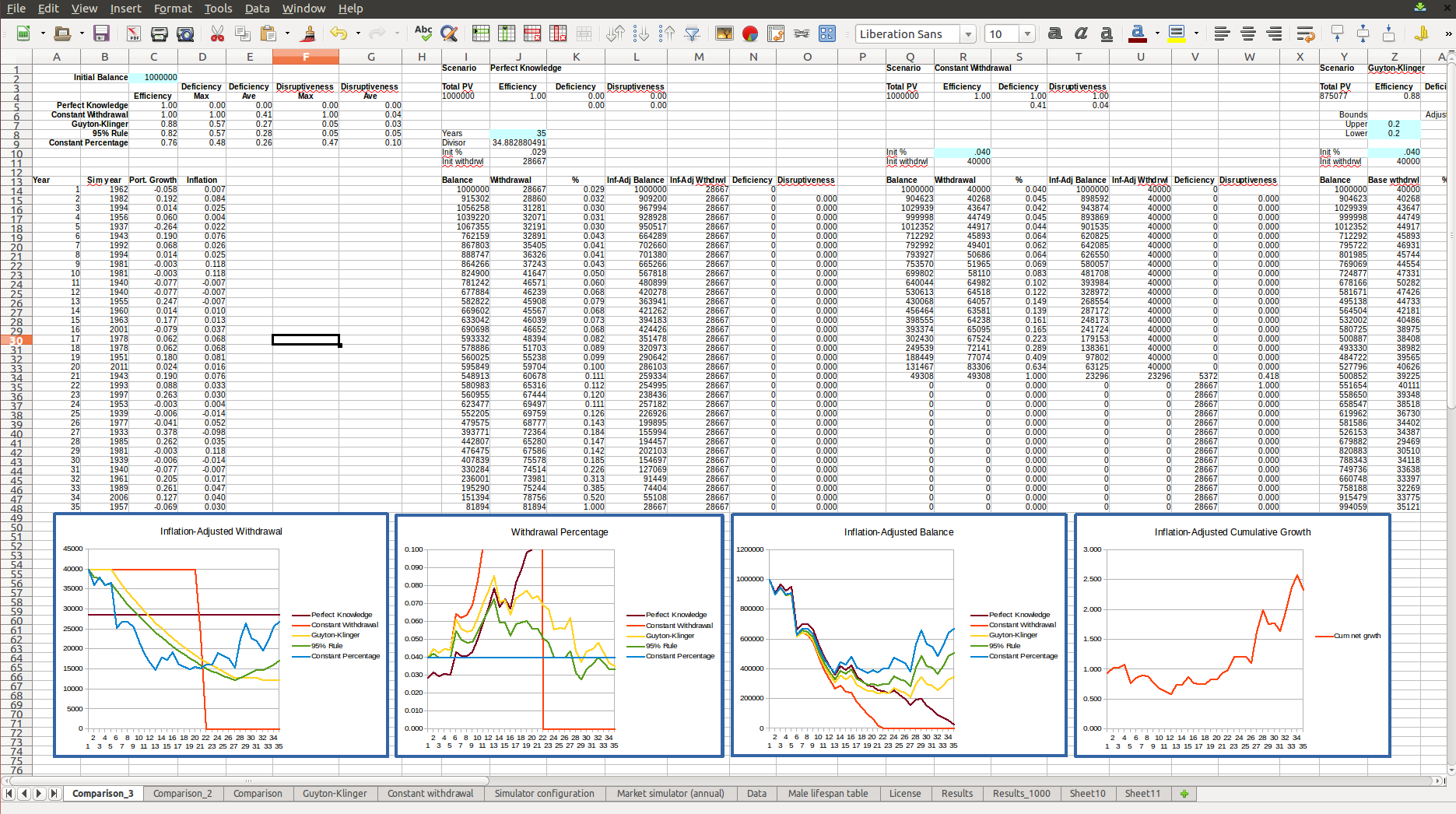
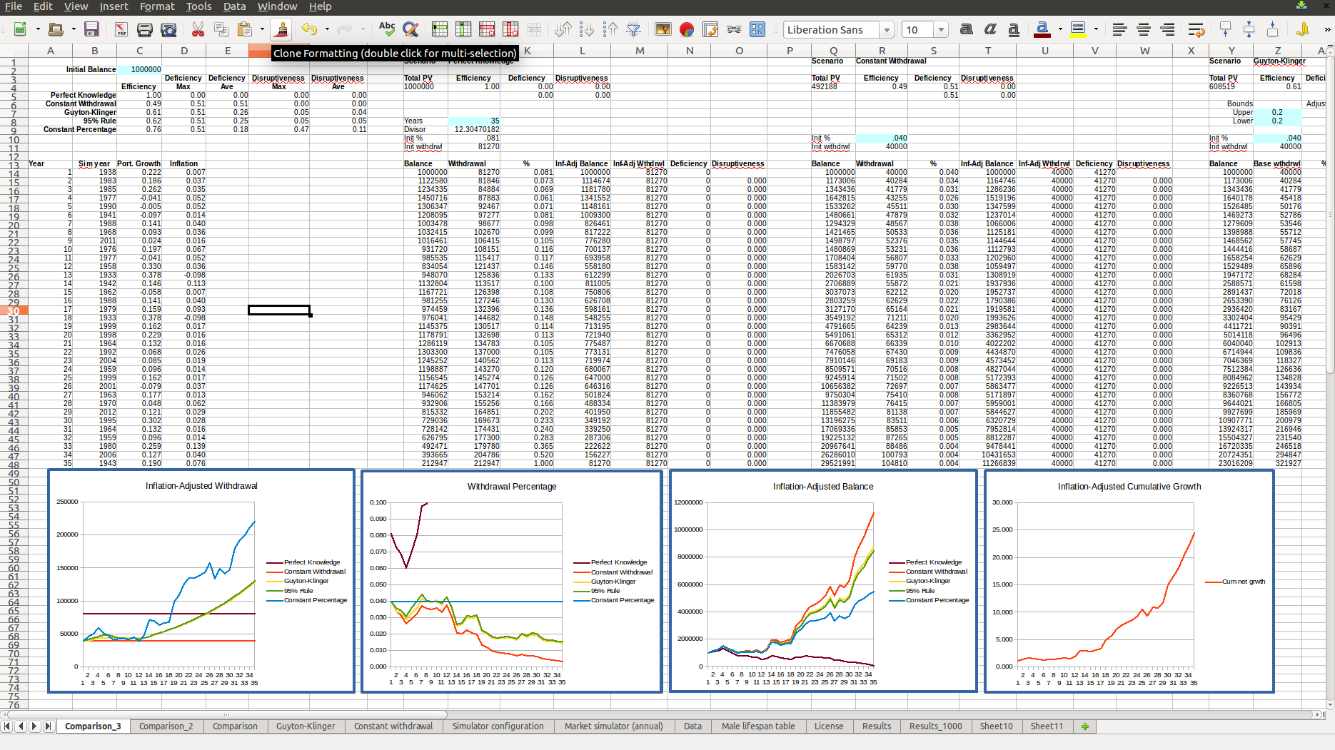
The graphs in the image below show how the schemes perform in several different ways. The first graph gives the annual withdrawal, adjusted for inflation so each year’s amount is in “today’s dollars”, i.e., with inflationary growth deducted. This allows direct comparison of spending power – a constant graph indicates constant spending power over the years. The second graph gives the percent of the portfolio that is being withdrawn each year. This can help indicate if the scheme is over-stressing the portfolio by taking out too large a chunk, or not taking out enough when times are good. The third graph gives the inflation-adjusted balance in the portfolio over time (adjusted to “today’s dollars”), while the fourth shows the aggregate inflation-adjusted growth rate.
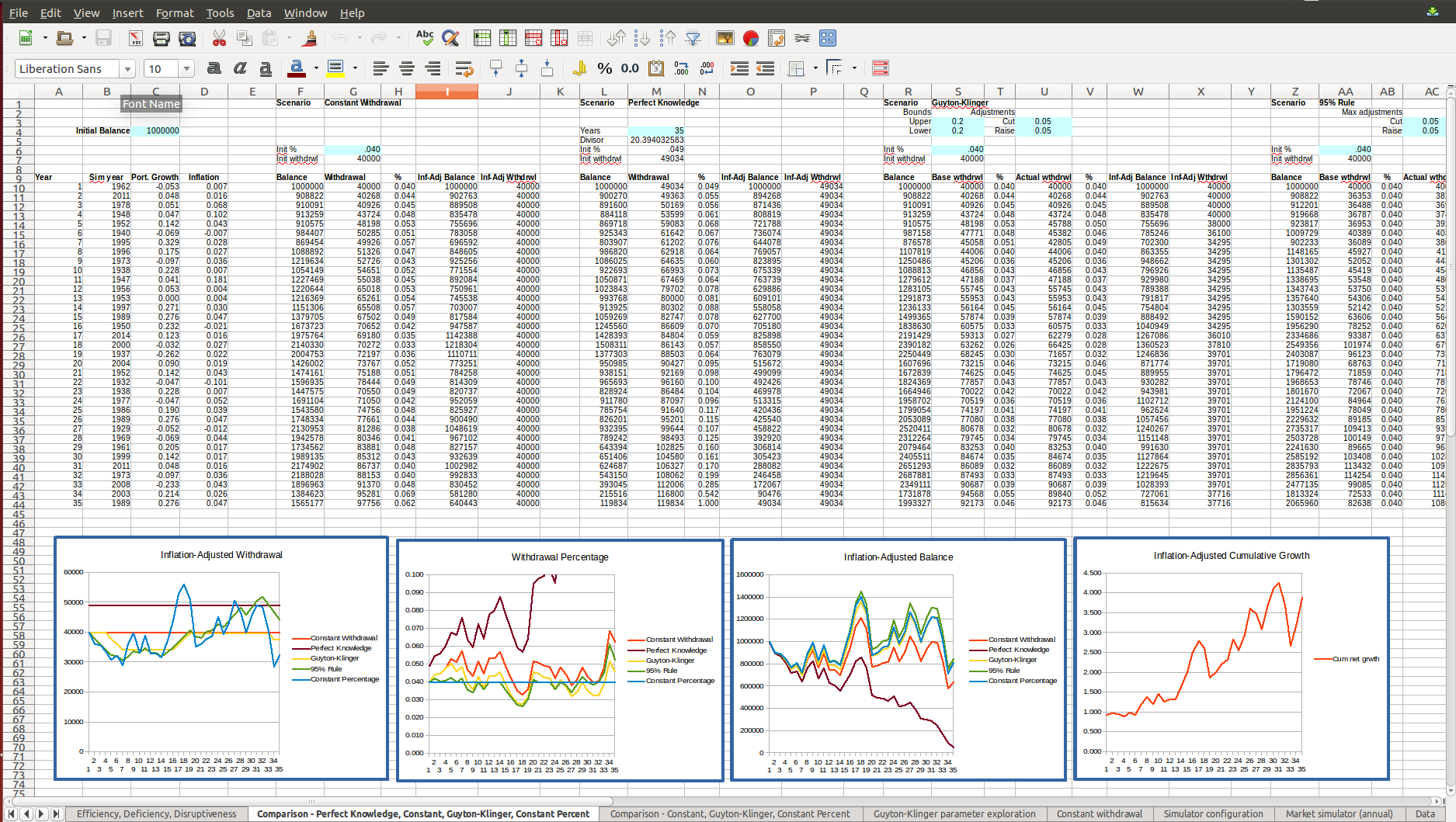
The annual-withdrawal graph shows that the Perfect Knowledge and Constant Withdrawal schemes take out a constant amount each year, as expected. The other schemes take out a varying amount over time, with the Constant Percent scheme showing the most year-to-year variation. The 95% Rule scheme tracks the Constant Percent scheme withdrawals, but lags due to the restriction that the change from year to year be no more than 5% from the previous year. And Guyton-Klinger similarly tracks the Constant Percent scheme, but with even less reactivity due to the fact that it only adjusts once the withdrawal percentage exceeds certain bounds (see the definition in this article), and the adjustment is held within specified limits (5% in the illustrations here).
The portfolio-balance graph shows the inflation-adjusted remaining portfolio over time. As expected, the Perfect Knowledge scheme balance declines until it is exhausted at exactly the end of the specified period. For the other schemes, we’d hope the balance wouldn’t fall to 0, at least not prematurely; for most market scenarios, that’s what we see, since the scenarios have been designed to try to keep us from running out of funds.
We can get some immediate qualitative sense of the benefits and drawbacks of each scheme from looking at these graphs over some different market scenarios; below are two, one “bad” low-growth scenario and one “good” high-growth scenario. Assuming we’d like our lifestyle to be as good as possible, i.e., we’d like our annual withdrawals to be as high as possible, then the higher the trace in the annual-withdrawal graph, the better for us. We can see that the adaptive schemes (Guyton-Klinger, 95% Rule, and Constant Percent) tend to reduce our spending when markets aren’t doing well, to help protect the portfolio, and augment our spending when the markets are booming. In some years, the annual amount can actually be higher than what we’d get from the Perfect Knowledge scheme, but this is balanced by years when the annual withdrawal is significantly less, so our annual withdrawals and thus lifestyle can vary quite a bit over time. The Constant Withdrawal scheme doesn’t impose such changes on us, but has the disadvantage of depleting the portfolio in some particularly bad market conditions and restraining our lifestyle unnecessarily in good conditions.
Efficiency, Deficiency and Disruptiveness
Beyond qualitatively observing the differences between the withdrawal schemes, how can we more objectively compare schemes to get a sense of which one is better, and specifically, better for us, based on our personal criteria for the “goodness” of a scheme? There are several quantities we can compute to help evaluate the schemes, in both specific market scenarios and statistically over a large number of scenarios.
Efficiency
One thing to look at is whether a scheme is providing us with as much of our assets as possible, or whether it leaves a large amount unspent at the end of the retirement period. To quantify this we look at the present value of the amount a scheme takes out for our use, i.e., the total of all withdrawals over the specified period, adjusted for growth. The higher this total amount, the more that a scheme has made available for us to use during our retirement. This is just the present value of an annuity, given specified payouts and known growth rates for each of the years. For the Perfect Knowledge scheme, this amount will exactly equal the starting balance; for the other schemes, this will generally be somewhat less depending on how much is left at the end of the retirement period.
We then define the efficiency of a scheme as the ratio of the total growth-adjusted withdrawal (present value) divided by the total withdrawal for the Perfect Knowledge scheme – i.e., how much the scheme provides as a fraction of the amount provided by the Perfect Knowledge scheme. The higher this ratio, the better a scheme has done to provide us funding for our retirement. This is the same as the Withdrawal Efficiency Rate used by Blanchett, Kowara and Chen. The efficiency will be 1 or less, since the present value of the annual distributions will always be less than or equal to the starting amount. It will be 1 if a scheme delivers the full amount, which is by design for the Perfect Knowledge scheme, but this will usually only happen for one of the other schemes if we prematurely run out of money. So while a higher efficiency is generally desirable, an efficiency of 1 usually is not!
Deficiency
Another thing we’d like to consider is how far below our ideal lifestyle a scheme might take us, both at maximum and on average. To do this we look at the times when a scheme has us taking out less than the Perfect Knowledge scheme would have us take out, and compute the ratio of the amount a scheme is deficient (the gap between the scheme’s withdrawal and the Perfect Knowledge withdrawal) to the amount the Perfect Knowledge scheme provides (which is constant over time). If a scheme has us taking out more than the Perfect Knowledge scheme, we use 0 for the gap and thus for the ratio. The maximum or average deficiency is then the maximum or average of these ratios. Thus a scheme which has a maximum deficiency of 0.43 in a scenario has us living at some point in time on just 57% of what the Perfect Knowledge scheme would have provided. By comparing deficiencies we can see whether one scheme tends to have us worse-off than another, either at some point or on average.
Note that the definition of deficiency is slanted toward the negative, in that we define the deficiency to be 0 when a scheme provides the more than the Perfect Knowledge scheme. We’re really looking at just the bad times, when we get less than we’d prefer, which is much harder to adapt to than when we’re getting more. We’d like to minimize the bad times; the good times pretty much take care of themselves.
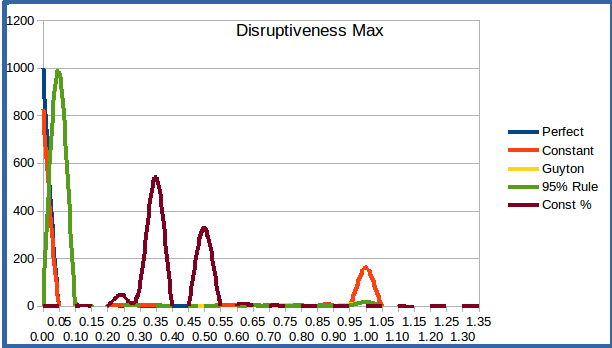
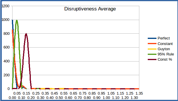
Disruptiveness
One additional measure to consider is how variable a scheme is – how much and how often we have to deal with swings in our annual income. We thus look at the percent change from year to year in the inflation-adjusted withdrawals, and define the maximum and average disruptiveness of a scheme to be the maximum and average of these percent changes. A Constant Withdrawal scheme generally has a disruptiveness of 0 – there are never any changes in annual income, adjusted for inflation (unless and until we run out of money). A Constant Percent scheme on the other hand has its annual withdrawal completely dependent on the portfolio balance and thus the market, and can swing almost as much as the market from year to year, which could be 30% or more in very turbulent times. This can be very disruptive to our lifestyle – hence the name.
Comparing the Schemes Quantitatively
With these definitions of efficiency, deficiency and disruptiveness, we can now compare the schemes in a quantitative sense. The associated spreadsheet (download below) computes and graphs these quantities for various simulated scenarios for a 35-year-long retirement period, so we can see how each performs under different market conditions. The values for efficiency, deficiency and disruptiveness can be seen in the spreadsheet images above, in the top left cells.
The spreadsheet also includes a macro, GenerateStats, that will iterate through 1000 scenarios, collecting the statistics from the tab Comaprison_3 for each scheme over each scenario, and then aggregating the values into averages and histograms in the output tab Results_1000. The result of 1000 such iterations is illustrated in the graphs below.
Efficiency
The efficiency averages over 1000 random market scenarios is in the following table. As expected, the Perfect Knowledge scheme provides perfect efficiency, while the others are somewhat less efficient since they generally strive to preserve some of the portfolio balance rather than trying to exhaust it on some schedule.
Average Efficiency Over 1000 Simulations, 35 year retirement period
| Perfect Knowledge | Constant Withdrawal | Guyton-Klinger | 95% Rule | Constant Percent |
| 1.00 | 0.68 | 0.72 | 0.74 | 0.76 |
But the averages don’t indicate how much the efficiency of a scheme varies from scenario to scenario – while the averages show the four schemes on the right to be relatively close in efficiency, they don’t indicate that some schemes do especially poorly under some conditions. A histogram showing the distribution of the efficiency values over the 1000 simulations can provide this information, as in the graphic below.
Efficiency Histogram, 1000 Simulations, 35-year retirement period
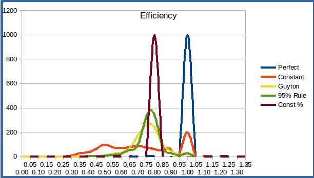
This shows that the Guyton-Klinger, 95% Rule, and Constant Percent withdrawal schemes generally give good efficiency, in the range of 0.65 to 0.85 over many scenarios, while the Constant Withdrawal scheme has a much broader span of efficiencies since it doesn’t adjust for increasing or decreasing portfolio balance. The only time the Constant Withdrawal scheme looks particularly good is when its efficiency is 1, which happens in about 20% of simulations; but as mentioned above this is an indication that we’ve distributed all of our funds, most likely prematurely. The single peak at around 0.80 for the Constant Percent scheme has a natural explanation: when we take out 4% of the remaining portfolio each year over a 35 year period, the present value of these distributions will just be 1 – (0.96)^35 = 0.76 of our starting portfolio, regardless of the growth rates since these are factored out in computing the present value.
Deficiency
The average and max deficiencies, and their averages and histograms, are shown below.
Max Deficiency, Average Over 1000 Simulations, 35 year retirement period
| Perfect Knowledge | Constant Withdrawal | Guyton-Klinger | 95% Rule | Constant Percent |
| 0.00 | 0.46 | 0.47 | 0.50 | 0.54 |
Average Deficiency, Average Over 1000 Simulations, 35 year retirement period
| Perfect Knowledge | Constant Withdrawal | Guyton-Klinger | 95% Rule | Constant Percent |
| 0.00 | 0.36 | 0.23 | 0.22 | 0.20 |
The table giving average deficiency shows that the Constant Withdrawal scheme has a much larger average deficiency than the other schemes. This is due to the fact that it doesn’t do anything to try to resolve the difference between what we’re currently taking out and the optimal amount. The other schemes try to adjust for an increasing balance, so reduce the deficiency on average. The Constant Percentage scheme is the most reactive to a changing portfolio balance, so it makes sense that it would on average reduce the deficiency best. But because it’s so reactive it can at times leave us with an even higher deficiency, as indicated in the max deficiency table.
The histograms reinforce this. Note the broad range of deficiency values for the Constant Withdrawal scheme, and the ~20% of scenarios in which the deficiency reaches 1, indicating that we’ve run out of money (corresponding exactly to those cases where the efficiency was 1).
Max Deficiency over 1000 Simulations, 35 year retirement period
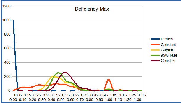
Average Deficiency over 1000 Simulations, 35 year retirement period

Disruptiveness
The average and max disruptiveness values, and their averages and histograms, are shown below.
Max Disruptiveness, Average Over 1000 Simulations, 35 year retirement period
| Perfect Knowledge | Constant Withdrawal | Guyton-Klinger | 95% Rule | Constant Percent |
| 0.00 | 0.14 | 0.06 | 0.06 | 0.31 |
Average Disruptiveness, Average Over 1000 Simulations, 35 year retirement period
| Perfect Knowledge | Constant Withdrawal | Guyton-Klinger | 95% Rule | Constant Percent |
| 0.00 | 0.01 | 0.03 | 0.05 | 0.12 |
These illustrate what we expect to see – that the Constant Percent scheme, with its direct tracking of the market through the portfolio balance, is the most volatile when it comes to year-to-year changes in income. The Guyton-Klinger and 95% Rule schemes are explicitly limited in the amount they will change the annual withdrawal, as seen in the 0.06 max disruptiveness for both; it’s greater than the 5% limit because in an additional ~1-2% of cases the schemes fail (run out of money before the end of the retirement term). The Guyton-Klinger scheme has less average disruptiveness, since it only changes the annual withdrawal in the instances where it exceeds the “guard rails”; in many years it won’t adjust at all (except of course for inflation, which is factored out in the statistics). The Constant Withdrawal scheme should have a disruptiveness of 0, since it keeps the inflation-adjusted withdrawal constant – except in those cases in which we run out of funds, at which point the disruptiveness rises to 1.00. This is what accounts for the non-zero max and average disruptiveness over the 1000 simulations – we do run out of funds in many scenarios with the Constant Withdrawal scheme.
These points are further illustrated by the histograms. Particularly interesting is the distribution of max disruptiveness for the Constant Percent scheme; the two large peaks indicate the most volatile year in the market simulation, and over the course of the 35 years in each simulation run it often occurred that there was at least one very good or bad year which caused the annual withdrawal to change drastically.
Max Disruptiveness over 1000 Simulations, 35 year retirement period
Average Disruptiveness over 1000 Simulations, 35 year retirement period
Conclusions
How can the above information be used to determine an “optimal” withdrawal scheme? Well, it depends on what’s most important to the retiree. Is high efficiency – eking the most out of the portfolio that it can deliver – key? Or is minimizing annual deficiency from the optimal “smooth” withdrawal more important? For many, finding a way to reduce disruptiveness will be even more important, since having a wildly gyrating lifestyle isn’t attractive to most.
From the above, if efficiency is key, and disruptiveness not a big issue, then the Constant Percent scheme might be the choice, as it gives the best efficiency despite its volatility. On the other hand, if a retiree is looking for a balance between efficiency and disruptiveness, then the Guyton-Klinger and 95% Rule schemes both perform well, with the 95% Rule having a slight edge in efficiency and the Guyton-Klinger scheme having slightly less volatility. The Guyton-Klinger and Dynamic Spending strategies also have a number of parameters that can be used to “tune” them to tweak one of the statistics if desired. (Recall that the 95% Rule is just a special case of the Dynamic Spending strategy that uses 5% as the withdrawal change limits from the previous year’s withdrawal – see this article for a detailed discussion.) And these are certainly not the only schemes that can be devised – there are lots of approaches to managing withdrawals from a portfolio. The efficiency, deficiency and disruptiveness measures can be used to compare these to find the one that’s right for a particular retiree. And a certified financial planner can help you to decide which is best for your unique circumstances.
Next Steps
One limitation of the analysis presented here is that the retirement period has been fixed at 35 years. Obviously, the length of the retirement period is the other big variable in retirement planning (along with market conditions). This is considered in the follow-up article Retirement Withdrawal Efficiency Revisited: Variable Lifespan and Annuities. This looks at efficiency when the length of the retirement period is varies along with market conditions, and considers the efficiency of life annuities as well.
Caveat
This information is presented as-is, with no guarantee as to accuracy or freedom from errors. This document and associated spreadsheet is intended as an observation for informational purposes only, and should not be used in retirement planning without cross-checking and correlating with other sources of information and consultation with a certified financial planner. I’m an enthusiast, not a professional, and being human I make mistakes. Your retirement funding is far too important to rely significantly on any unvalidated information!
Spreadsheet Simulator Download
The simulator is open-source software licensed under the Gnu General Public License v2. This gives you the right to use the simulator for your purposes, and adapt it (create a derived work) as you see fit as long as you make the new spreadsheet available for other users. See the link above for license details.
Data source for economic data used in the simulator
Historical returns: Stocks, T.Bonds & T.Bills with premiums, Aswath Damodaran, Stern School of Business, New York University.
References
Optimal Withdrawal Strategy for Retirement Income Portfolios, 2012, Blanchett, Kowara, Chen, Morningstar Investment Management.
New Math for Retirees and the 4% Withdrawal Rule, New York Times, May 8, 2015.
A Better Way to Tap Your Retirement Savings, Wall Street Journal, May 31, 2015.
Using Decision Rules to Create Retirement Withdrawal Profiles, William Klinger, Journal of Financial Planning, August 2007.
Work Less, Live More, Bob Clyatt, 2007.
A rule for all seasons: Vanguard’s dynamic approach to retirement spending, Michael A. DiJoseph, Colleen M. Jaconetti, Zoe B. Odenwalder, and Francis M. Kinniry Jr., Vanguard Research, March 2017.
Articles in this series
-
Life Tables and Retirement Planning
-
Retirement Withdrawal Strategies: Guyton-Klinger as a Happy Medium
-
Variable Withdrawal Schemes: Guyton-Klinger, Dynamic Spending, and CAPE-Based
-
Comparing Retirement Withdrawal Schemes: Efficiency, Deficiency, and Disruptiveness
-
Retirement Withdrawal Efficiency Revisited: Variable Lifespan and Annuities
-
Annual or Monthly Withdrawal? Dollar Cost Averaging in Retirement
-
Over-valued, Under-valued, or Just About Right? Assessing Retirement Portfolios in Current Conditions