In a previous article, the quantities efficiency, deficiency and disruptiveness were defined for comparing retirement withdrawal schemes.In short, efficiency measures how much of our portfolio is delivered back to us before the end of the retirement period; deficiency measures how much a scheme falls short of delivering the optimal annual amount that an “ideal” scheme would provide (discussed below); and disruptiveness measures how much of a year-to-year swing we might have to endure from schemes that provide variable annual withdrawals in response to market changes.

These quantities utilize comparison with an ideal “perfect knowledge” scheme, which uses information about future market conditions to determine the optimal constant inflation-adjusted withdrawal that could be taken annually from a portfolio so that all the retirement funds would be used up exactly at the end of a specified retirement period (taken as 35 years in the previous article). This scheme was first introduced in a paper by Blanchett, Kowara and Chen, who also introduced the concept of the efficiency of a withdrawal scheme. Of course, the perfect knowledge withdrawal scheme is purely hypothetical – we don’t know the future market conditions, and this is one of the principal difficulties in retirement planning.

The other factor that complicates retirement funding is deciding what to use for the retirement period, i.e., the length of time we’ll be in retirement, which is determined by lifespan. Clearly, this is the other big unknowable, and will affect the efficiency of the retirement withdrawal scheme – for any given withdrawal scheme, the longer our lifespan, the more the scheme will deliver to us from our portfolio, and thus the higher the efficiency – and conversely for a shorter lifespan. This article revisits efficiency of withdrawal schemes when variable lifespans are taken into account. We don’t address deficiency or disruptiveness, as these are more dependent on market conditions than longevity, though they will vary somewhat based on lifespan – the longer the lifespan, the more opportunity there is for the market to experience a disruptive event.

Perfect Knowledge with Variable Lifespan

The perfect knowledge scheme as used in the previous article used knowledge of market conditions over the assumed 35-year retirement period and computed the constant inflation-adjusted annual withdrawal that could be made so the funds were exactly exhausted at the end of the 35-year term. But there’s nothing special about using a 35-year term – for any other given retirement period length, we can do the same.

Simulation with Variable Lifespan

We thus repeat the simulations used in the previous article, but instead of using a fixed 35-year retirement term, we randomly select a period using probability tables for lifespan, as presented and discussed in another article on this website. We thus select both a set of market conditions based on historical data and a randomly-selected retirement period using  the probability distribution from the life tables, and determine the efficiency, deficiency and disruptiveness for these conditions and retirement term. Running multiple simulations, we can then study the effect of both variable market conditions and lifespan on these parameters.

Of course, lifespan probabilities depend on our current age; the probability is considerably higher that we’ll live an additional 10 years if we’re currently 40 than if we’re 90. The probabilities also depend on gender – women at any age generally live longer than men of the same age – and on country – lifespan in different countries varies significantly. We do the simulations for a 65-year-old male in the US.

Simulation Results

As mentioned above, we focus just on efficiency, as this is the parameter that is most affected by lifespan. We first look at the average efficiency over all the simulation runs for the retirement withdrawal schemes considered.

Average Efficiency

We compute the average efficiency of a withdrawal scheme by averaging its efficiency over 1000 simulation runs with both varying market conditions and lifespan.

Average Efficiency Over 1000 Simulations, randomly-selected retirement period

Perfect Knowledge	Constant Withdrawal	Guyton-Klinger	95% Rule	Constant Percent
1.00	0.56	0.58	0.61	0.60

 

From the above, we can see that the efficiency of all of the retirement schemes considered is around 60% when variable lifespan is taken into account. This means that, on average, each scheme would be expected to return about 60% of the value of the portfolio over the course of a retirement lifespan (using present value for future withdrawals). There is relatively little variation between the schemes regarding efficiency – only about 5%. But remember that there are other factors that may make one scheme more desirable than another, as discussed in the previous article, especially the probability of failure (running out of funds before the retirement term is ended).

How does this compare with the previous simulations for a fixed retirement term? For reference, we include the tables from the previous article, which used a fixed 35-year retirement period.

Average Efficiency Over 1000 Simulations, 35 year retirement period

Perfect Knowledge	Constant Withdrawal	Guyton-Klinger	95% Rule	Constant Percent
1.00	0.68	0.72	0.74	0.76

 

We can see that the efficiencies are higher for a 35-year term than for a variable term. This can be easily explained by noting that the expected lifespan for a 65-year-old man in the US is about 18 years according to life tables. With this shorter period being the average lifespan, we would expect the efficiency of a scheme to be lower on average as there would be less time to return the assets.

Distribution of Efficiency Values

As before, the averages don’t indicate how much the efficiency of a scheme varies from scenario to scenario – while the averages show the four schemes to be relatively close in efficiency, they don’t indicate that some schemes do especially poorly under some conditions. A histogram showing the distribution of the efficiency values over the 1000 simulations can shed some light, as in the graphic below. We include the histogram from the previous fixed-term simulation for comparison.

Efficiency Histogram, 1000 Simulations, randomly-selected retirement period

 

Efficiency Histogram, 1000 Simulations, 35-year retirement period

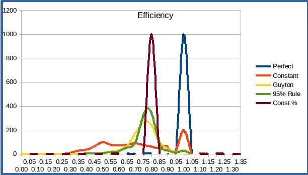
We can immediately see that the efficiency values vary much more widely with a variable-length retirement term than with a fixed-length term. This makes sense given the observations above regarding the average values. The shorter the retirement term, the lower the efficiency, since the length of time directly affects how many annual payments are delivered and thus how much of our funds we can expect to get back. With randomly selected lifespans, we include both shorter (lower efficiency) and longer (higher efficiency) timespans.

This again shows that the Guyton-Klinger, 95% Rule, and Constant Percent withdrawal schemes generally give good efficiency, while the Constant Withdrawal scheme has a broader span of efficiencies, especially at the low end. One anomaly is that the Constant Withdrawal scheme has a pronounced (small) peak at efficiency 1.00; but as mentioned before this is an indication that we’ve distributed all of our funds, in most cases prematurely. This is almost always a very undesirable outcome  since it usually means we’ve run out of money, but it makes the average efficiency of the Constant Withdrawal scheme look better than we might want to regard it. We can thus re-analyze the efficiency data, excluding any data points in which a scheme runs out of funds. This drops the average efficiency of the Constant Withdrawal Scheme to 53%, and eliminates the small “hump” at efficiency 1.00 in the histogram. (The other schemes’ average efficiencies and histograms aren’t significantly affected when failures are eliminated, as there are very few times that they actually run completely out of funds in the simulations. That’s one of the reason these adaptive schemes are generally much more desirable than a constant-withdrawal approach.)

Pension Funds and Annuities

It’s worth noting that the individual investor is at a significant disadvantage to a pension fund manager in one important respect. The fund manager, handling funds for many retirees, doesn’t have the problem of unknown lifespan, at least if he has a large number of retirees in his fund. While any individual in the fund has a completely unknowable lifespan, the population as a whole will statistically (with very high probability) have a distribution of lifespans that matches the probability distribution in the life tables. He thus doesn’t have the unknown-longevity problem that the individual investor has. He knows just how much to pay out based on the average lifespan, and knows that the average is highly unlikely to vary much from the expected (as long as he has enough people in the fund). Those who live longer are balanced out by those who live shorter – longevity problem solved.

How can individual investors take advantage of this “lifespan pooling”? Well, this is essentially what is provided by an annuity. You buy in to the annuity (contribute your funds to the annuity pot), and then get paid throughout your life based on your average expected lifespan. If you live longer than expected, you continue getting paid, courtesy of those unfortunates who pass away early.

Of course, there are lots of caveats/drawbacks to the use of annuities. First, you generally lose access to your money – it becomes part of the annuity “pot”. With some annuities, you can reclaim some of your funds if you need them in an emergency, but you pay a penalty for this. Also, your heirs generally lose out, as any leftover funds when you pass away are kept by the annuity fund. This can be especially significant if you pass away early. There are some annuity plans that allow for some of the funds to be returned to your heirs pro-rated on your lifespan, but you generally pay for this in reduced payments during your lifetime. And plain-vanilla annuity payments aren’t adjusted for inflation – you get a fixed amount annually for life, regardless of inflation, which can take a real toll, especially if you live long through turbulent times. You can find inflation-adjusted annuities, but you pay for this feature, again in reduced annual payments. And the amount you get annually is fixed when you purchase the annuity, generally stated as some percentage of the purchase value; these days it’s something like 6% for a 65-year-old male. Whatever the market conditions, you get 6% of your initial investment every year. There are annuities that pay out a different amount based on market performance, but – you guessed it – you generally pay for this feature too.

There are more flavors of annuity than there are flavors of ice cream, which can make it hard to understand if they’re a good deal or not. But the bottom line is, you’re really handing your nest egg to someone else, in exchange for a lifetime paycheck. The pros? You don’t have to worry about outliving your assets (which you don’t have any more anyway); you don’t have to worry about investment decisions (it’s not your problem because it’s not your money any more); and you don’t have to worry about varying market conditions (as long as the annuity provider stays afloat). The cons? Well, your money’s gone – no longer in your control. And looking at current annuity rates, given that the life tables tell us a 65-year-old man has an average lifespan of about 18 years, the total amount he would expect to get back on average would be 18 * 6% = 108% of his initial investment – but that’s NOT present value, i.e., adjusted for either inflation or market returns. We look at how this might compare to other schemes in the next section, where we consider the efficiency of an annuity.

Efficiency of some Common Annuities

We can look a little deeper into the pros and cons of annuities using the same measures we’ve used for other retirement withdrawal schemes – namely, the efficiency, deficiency and disruptiveness. We’ll look at just two of the most common annuity types:

• Plain life annuity (fixed payouts over the retiree’s lifespan)
• Inflation-protected life annuity (payouts increasing by a fixed percentage each year to compensate for the possibility of inflation)

It’s worth noting that basic inflation-protected annuities don’t try to adjust using the actual inflation rate; they just increase the payments each year by some fixed percentage (say 3%) to help compensate for any inflation that might occur. If the inflation rate is less than this fixed percentage, you win – your annual payouts will have more buying power over time – and if it’s less, you lose. The insurers greatly prefer this to adjusting using the actual inflation values, since it eliminates all the uncertainty (for them) regarding inflation.

Simulations for Annuities

We use the variable-life simulations to investigate the performance of these two types of annuities, using currently available rates as provided by the New Retirement annuity calculator for a 65-year-old male:

• Plain life annuity: 6.4452%
• Inflation-protected annuity with 3% annual increase: 4.71%

This means that for a $1,000,000 investment, you’ll receive $64,452 annually from the plain life annuity, or $47,100 initially, incremented by 3% each year, from the inflation-protected annuity. The inflation-protected annuity payments start out lower, but increase over time.

Simulation Results

We look primarily at the efficiency of an annuity scheme – what fraction of the portfolio (present value) is returned to the retiree in his lifetime. The table below shows the results from 1000 market simulations with variable lifespan.

Average Efficiency Over 1000 Simulations, randomly-selected retirement period

Perfect Knowledge	Constant Withdrawal	Guyton-Klinger	95% Rule	Constant Percent	Annuity	Annuity (Inf prot)
1.00	0.56	0.58	0.61	0.60	0.71	0.67

 

Purely from the perspective of our previous definition of efficiency – how effectively does the withdrawal scheme deliver the funds in the portfolio to the retiree over the course of his lifespan – the annuity options look pretty good, delivering a larger fraction on average than the other withdrawal schemes. But there’s a big caveat: while the annuity delivers a larger fraction of the funds to the retiree while he’s alive, there’s nothing left over when he dies – the remainder stays in the annuity “pool” to fund others’ retirements. For the other schemes, whatever’s left over is yours to allocate as you see fit (through your will). If we had included the legacy in the calculation, then the efficiency of all the other schemes would have been be 1, since all your money is accounted for either through distribution during your lifetime or as an inheritance. But that’s not what we set out to measure – efficiency was defined to determine how well the portfolio delivers for the retiree during his lifetime.

As with the other withdrawal schemes, the efficiency of an annuity varies, with lifespan (the longer the lifespan, the more an annuity pays you), but also with market conditions. The latter occurs because our definition of efficiency uses the present value of the distributions, which is dependent on the market conditions. The efficiency histogram below includes the two annuity schemes along with the others. One interesting feature is that there are scenarios where an annuity can deliver efficiency above 1.0, as seen by the small rise to the right of 1 on the histogram. This makes sense: since the annuity terms (payout rate and inflation adjustment) are set up front, an annuity can pay out more than the perfect-knowledge scheme in cases where the market is weaker over the lifespan than it was when the annuity terms were established.

Efficiency Histogram, 1000 Simulations, randomly-selected retirement period, including annuities

We also take a quick look at the other measures that were previously investigated to compare the withdrawal schemes, deficiency and disruptiveness. These are found to be similar to the other schemes, as seen below. It might seem odd that there’s any disruptiveness with an annuity – after all, it’s either a constant series of payments, or a constantly-increasing series in an inflation-protected annuity. But remember that neither of these takes into account the real value of inflation, so the true inflation-adjusted amount you receive can drop significantly in a year when inflation is high.

Average Deficiency Over 1000 Simulations, randomly-selected retirement period, including annuities

Perfect Knowledge	Constant Withdrawal	Guyton-Klinger	95% Rule	Constant Percent	Annuity	Annuity (Inf prot)
0.00	0.45	0.40	0.38	0.35	0.38	0.36

 

Average Disruptiveness Over 1000 Simulations, randomly-selected retirement period, including annuities

Perfect Knowledge	Constant Withdrawal	Guyton-Klinger	95% Rule	Constant Percent	Annuity	Annuity (Inf prot)
0.00	0.00	0.03	0.05	0.12	0.04	0.03

 

To Annuitize or Not To Annuitize…

So if your goal is to use up all your savings as best you can, and you’re not interested in leaving any sort of legacy, than an annuity seems to provide a somewhat more efficient delivery of your assets back to you over your lifespan. And one primary advantage of an annuity is that you won’t run out of money, since the payments will continue throughout your lifetime, regardless of how long you live. Plus you’re insulated from market ups and downs – it’s not your problem (as long as the annuity fund is managed well enough not to go under). However, since there’s either no inflation adjustment, or a fixed adjustment, you might find your lifestyle impacted in times of high inflation. And your money is no longer yours, so if you need it for an emergency, you may not be able to get the remainder back (or will pay a steep penalty to do so).

One approach that’s advocated by some advisors is to annuitize an amount that’s enough to cover your basic needs, and keep the rest of your assets invested in the market. This way even if something catastrophic happens (your asset manager turns out to be an acolyte of Bernie Madoff), or something remarkable happens (you live to be 120), you won’t be left destitute; but you also get to benefit from general market growth with the invested portion of your portfolio.

But of course, if you are a US citizen, you already have an annuity in the form of Social Security. And this is the best kind, in that it’s adjusted annually using the real value of inflation, so the payments should (in theory) maintain constant buying power over the course of your lifetime. You should certainly factor that into any planning – you may already have an annuity that meets the basic-needs test. And though we hear daily that Social Security funding is troubled, and will run out of money, and payments will have to be drastically cut, we’ve been there before, and additional funding has always been found to make the system solvent, so I’m not too worried. After all, imagine the future for a politician who cuts the retirement safety net of the nation’s elderly… I wouldn’t want to be him at the next Thanksgiving dinner.

Conclusion

Simulations show that the efficiency of the withdrawal schemes when variable lifespan is taken into account is reduced somewhat from what was seen with a fixed-term retirement period. However, this can be easily explained by observing that the 35-year length of the fixed-term retirement period considered previously was considerably longer than the expected lifespan of the assumed 65-year-old male in the variable lifespan trials. We can also see that the adaptive withdrawal schemes (Guyton-Klinger, 95% Rule, and Constant Percentage) still provide better efficiency than a constant withdrawal scheme, both on average and in most cases (as indicated by the histograms). This helps to confirm that the adaptive schemes are preferable in this regard (as well as for many other reasons discussed in previous articles).

As far as overall efficiency of utilization of retirement funds is concerned, we see that on average we can expect to have about 60% of our accumulated savings returned to us over the course of a retirement – more if we live longer, less if our lifespan is shorter than average. While 60% doesn’t sound like a great return on our assets, it’s worth remembering that this is in an environment in which the two important factors (market conditions and longevity) are unknowable. While it’s worth continuing to investigate ways that this might be improved (I’ll certainly keep looking), it might be the best one could hope for.

The exception to the 60% return is the case of annuities, which can provide a return of nearly 70%, and provide guaranteed income throughout life. But this comes at the cost of losing control of your money and the return of any remaining assets at the end of life. Losing on average the remaining 30% of your assets is a pretty high price to pay for a modest increase in efficiency during retirement, in my view.

Caveat

This information is presented as-is, with no guarantee as to accuracy or freedom from errors. This document is intended as an observation for informational purposes only, and should not be used in retirement planning  without cross-checking and correlating with other sources of information and consultation with a certified financial planner. I’m an enthusiast, not a professional, and being human make mistakes. Your retirement funding is far too important to rely significantly on any unvalidated information!

Acknowledgements

Thanks to Jonathan Kandell for suggesting incorporating variable lifespan based on life table probabilities into the simulations.

Resources

• Annuity estimator from New Retirement
• Spreadsheet used to run simulations for this article

References

Optimal Withdrawal Strategy for Retirement Income Portfolios, 2012, Blanchett, Kowara, Chen, Morningstar Investment Management.

Articles in this series

• Life Tables and Retirement Planning

• Retirement Withdrawal Strategies: Guyton-Klinger as a Happy Medium

• Variable Withdrawal Schemes: Guyton-Klinger, Dynamic Spending, and CAPE-Based

• Comparing Retirement Withdrawal Schemes: Efficiency, Deficiency, and Disruptiveness

• Retirement Withdrawal Efficiency Revisited: Variable Lifespan and Annuities

• Annual or Monthly Withdrawal? Dollar Cost Averaging in Retirement

• Over-valued, Under-valued, or Just About Right? Assessing Retirement Portfolios in Current Conditions