One of the most important topics in retirement funding for those with IRAs or 401ks is withdrawal: how much can you take from your portfolio each year over the course of retirement without depleting the portfolio too soon? The well-known 4% scheme is one approach – determine the first year’s withdrawal as 4% of the starting portfolio balance, and then take each subsequent year’s withdrawal by adjusting the previous year’s withdrawal for inflation. This is known as a “constant withdrawal” scheme, as discussed in this article. This has the nice property of providing constant inflation-adjusted withdrawals, so spending power stays the same over the course of retirement – unless of course the portfolio runs out of money because the withdrawals are too high to be supported because of poor market conditions. The “4%” in the 4% rule was selected from historical data – it gave the maximum constant inflation-adjusted amount that could have been withdrawn from a portfolio of roughly 60% large-cap stocks and 40% bonds without depleting the portfolio over a 30-year period for any retirement period that started between 1928 and 1991. But as they say, past performance is not a guarantee of future results. And running out of money is the one result that really needs to be avoided.
The 4% method has been extensively studied, and enhanced using additional economic information. One principal focus has been on the 4% figure itself. Is 4% really the optimal starting amount to take from the portfolio? It was selected as the highest starting withdrawal rate that would keep the portfolio from running dry over all the historical scenarios. As such, it was the safest, most conservative value, often called the “safe withdrawal rate” in discussions, that would keep the portfolio from running dry even during the most challenging historical market conditions. While running out of funds is definitely the most important factor to consider in determining the amount to withdraw each year, one significant downside to the 4% rule is that in most of the historical scenarios, it was actually considerably less than could have been safely withdrawn, and thus the portfolio would have ended up with a lot of unspent funds. In many of the historical cases, an investor could have set the initial portfolio withdrawal at 5%, 6% or even 7%, and rosy market conditions over the retirement years would have grown the portfolio enough to support this. The problem is that you wouldn’t have known you were in one of the rosy scenarios until the retirement period was over, at which point a 4% initial withdrawal would have left you with a large remaining portfolio. And if you selected a higher initial withdrawal and happened to be in one of the challenging scenarios, you’d have run out of money.
One interesting thing to note is that Bill Bengen, the originator of the 4% rule, has himself updated the 4% rule to be the 4.7% rule – that is, the safe initial withdrawal rate he he now advocates is 4.7%, not 4%. That’s due to in part assuming that a retiree’s portfolio uses a broader range of investments than just large-cap stocks and treasury bonds. He also assumes that an investor won’t just blindly withdraw funds until the portfolio is exhausted, but will cut back if things look dicey. Of course, if and when to cut back, and by how much, then become the key questions. Some approaches to this are discussed later in this article. And in some circumstances even a 4.7% initial withdrawal rate might be low and leave a lot on the table.
4%? 5%? 6%? How to decide?
To address the question of how to choose an initial withdrawal rate that’s neither too high nor too low, a number of researchers have looked more closely at indicators that might help predict whether you were likely to encounter good market conditions or weak ones when you start retirement withdrawals. While a typical retirement might span 30 years or more, the first decade is generally seen as critical in determining whether funds will last, and thus any way to predict if the next 10 years of market returns are likely to be above-average or below-average could be very useful in determining how large the initial withdrawal should be. One natural thing to consider is whether the market is over-valued or under-valued on the date of retirement. If it’s over-valued, i.e., we’re in some sort of market bubble, the expectation is that the market will fall in the short term, and that the overall growth over the next decade or so will be below average as the bubble deflates and recovery begins. Similarly, if it’s under-valued, i.e. the market is in a trough, maybe following a bubble, then we’d expect growth from that point to be even more robust than usual as the market digs itself out of the hole. Another article on this website provides a simplistic look at whether markets are over- or under-valued at present, by looking at historical data and trying to identify bubbles and troughs.
But a significantly better and more quantitative approach is to look at stock price-to-earning (P/E) ratios, or the smoothed cyclically-adjusted price/earnings (CAPE) developed by economist Robert Shiller. By looking at the price-to-earnings ratio of a particular stock, we’re looking at what a share of the stock costs divided by the earnings it provides us as investors, in terms of how much each share costs for each dollar of annual revenue it provides. If the P/E ratio for a stock is 10, that means that for every $10 we invest in shares we’ll generate $1 in annual earnings. A $1 return on a $10 investment is a 10% return rate – not bad at all. On the other hand, if the P/E ratio of a stock is 25, that means you need to spend $25 to get $1 in annual revenue, for a 4% return rate – less appealing. And at a P/E ratio of 33, the return is only 3%. Add to this the fact that stock prices are quite volatile, subject to both changing business conditions and (especially today) random investor likes and dislikes, and that 3% return seems mighty risky. While these earnings are usually not returned directly to the investor as dividends, being instead invested in expanding operations or stored as a cash reserve, it still represents an additional $1 worth of value that the shareholder owns (and could presumably recoup by selling the shares at a profit). In this way, it indicates the expected growth rate of the share price. If a $10 share generates $1 in revenue in the course of a year, you could reasonably expect to be able to sell the share for $11 at the end of the year, for a growth rate of 10%. The $33 share that generates $1 in revenue really ought to be worth $34 at year’s end, for a growth rate of 3%.
The CAPE applies the same logic to a collection of stocks, such as the S&P 500. Its value can thus give us a sense of what we might expect for the growth rate of a holding of these stocks in the coming years. If the CAPE is 10, we might expect a 10%, i.e., above-average, growth rate; if it’s 25, we might expect a 4% or below-average growth rate.
Researcher Michael Kitces has used historical CAPE data to determine what a safe initial withdrawal rate should be based on the CAPE value in the year of retirement. The lower the CAPE, the higher the initial withdrawal can be, since this implies the market is likely under-valued and likely to have a higher return over the next decade or so. For a high CAPE, the assumption is that the market is over-valued and will have a lower near-term return, and thus a lower initial withdrawal is called for. Kitces provides the following guidance.
Kitces’ suggested withdrawal rates based on CAPE
| CAPE at retirement | Initial withdrawal rate |
| >20 | 4.5% |
| 12 – 20 | 5.0% |
| <12 | 5.5% |
Bill Bengen, the originator of the original 4% (now 4.7%) rule, has taken Kitces’ work and included inflation as an additional predictor of performance, resulting in a more detailed recommendation of initial withdrawal rates given the CAPE and inflation rate in the year of retirement. An expanded version of several tables developed by Bengen is below.
Bengen’s suggested initial withdrawal rate as function of CAPE and inflation in year of retirement
| CAPE | < -5% inflation | -5% to -2.5% inflation | -2.5% to 0% inflation | 0% to 2.5% inflation | 2.5% to 5% inflation | > 5% inflation |
| 5-6 | 13% | |||||
| 6-7 | 13% | 10% | ||||
| 7-8 | 10% | 10% | ||||
| 8-9 | 10% | 9% | 8.5% | |||
| 9-10 | 9% | 8.5% | 7.5% | 9% | 8.5% | |
| 10-11 | 9% | 8.5% | 7.5% | 7.5% | 7.25% | |
| 11-12 | 8% | 7.5% | 7% | 7.5% | 7.25% | |
| 12-13 | 8% | 7.5% | 7% | 6.75% | 6.5% | |
| 13-14 | 7% | 7% | 6.5% | 6.75% | 6.5% | |
| 14-15 | 7% | 8% | 7% | 6.5% | 6.5% | 6% |
| 15-16 | 7% | 8% | 7% | 6% | 6.5% | 6% |
| 16-17 | 7% | 8% | 7% | 6% | 6% | 5.5% |
| 17-18 | 7% | 8% | 7% | 6% | 6% | 5.5% |
| 18-19 | 7% | 7% | 6% | 5.5% | 4.75% | |
| 19-20 | 7% | 7% | 5.5% | 5.5% | 4.75% | |
| 20-21 | 7% | 7% | 5.5% | 5% | 4.5% | |
| 21-22 | 7% | 6% | 5% | 5% | 4.5% | |
| >22 | 6% | 6% | 5% | 4.5% | 4.5% |
The rationale for these approaches to determining the safe initial withdrawal rate is discussed in an article by Bill Bengen in Financial Advisor magazine. It involves looking at historical data and determining what the maximum initial withdrawal rate would have been to keep from running out of money over a 30-year period if a retiree had retired in some past year. These tables have been developed to indicate the initial withdrawal rate that was safe in the past. One caveat is that there is relatively limited data – there are relatively few 30-year stretches covered by the data, so there aren’t a lot of examples in which, say, the CAPE was between 15 and 16 and the inflation rate was between 2.5% and 5%. While the recommendations above accurately reflect what would have been safe for those examples available, there’s not a lot of examples to test whether they would work in other cases where the parameters were similar. As mentioned before, the past is not a guaranteed predictor of the future, especially in investing, and having little data to go on makes the connection even weaker. Choosing a too-high withdrawal, and sticking to it, is a way to bring about the one fate every retiree wants to avoid.
Adapting to Change
The main problem with the 4% method and its updated cousins is that it completely ignores the current portfolio value and market conditions once withdrawals have begun, just blindly taking out the same inflation-adjusted amount each year regardless of the size of the remaining portfolio. In truth, no real investor would do this – if the portfolio balance were down due to bad market conditions, we’d all cut back on our withdrawals. And if the portfolio started to balloon due to good conditions, we’d all want to take advantage by withdrawing more and improving our lifestyle. The obvious question is, how much more or less should we take, and under what circumstances? Variable-withdrawal schemes address this by providing algorithms that vary the withdrawal each year based on the current portfolio value and/or market conditions. This article discusses and compares several such schemes.
The Guyton-Klinger Method
The Guyton-Klinger variable withdrawal scheme is one of the more widely discussed and analyzed methods. It has been discussed at length in another article on this website. The Guyton-Klinger approach tries to avoid depleting the portfolio by making sure withdrawals aren’t more than the portfolio can sustain (and increasing them if the portfolio is likely to balloon). A short description is as follows: start with an initial withdrawal (say, 4%), and then in each subsequent year, adjust the previous year’s withdrawal for inflation (just like the 4% rule), BUT adjust this further by giving yourself a “raise” or a “pay cut” if the amount to be withdrawn is “too small” or “too large”. The assessment of “too small” or “too large” is done by looking at the inflation-adjusted withdrawal as a percentage of the current portfolio value: if it would be too large a percentage (say, 5%), take a pay cut before withdrawing; if it’s too small a percentage (say 3%), give yourself a pay raise. The “too high” and “too low” percentages are often called the “guardrails” in the literature – if your withdrawal would go outside the guardrails, the adjustments try to “steer you back” into the optimal (and safe) withdrawal-percentage zone. As seen in the previous section, taking a too-high-percentage withdrawal risks depleting the portfolio early, and taking too small a percentage leaves a large balance that could otherwise be used.
The decision as to what the initial withdrawal percentage is, what to use as the upper and lower guardrail percentages, and what the pay cut and raise should be (usually expressed as a percentage) are parameters that must be selected to use the method, which gives a lot of flexibility.
The Dynamic Spending approach
Vanguard has presented an alternative variable withdrawal strategy they call Dynamic Spending. It is similar to the Guyton-Klinger method, but has a different focus. The Vanguard approach is a modification of the “constant percentage” withdrawal scheme, also discussed in the article mentioned above. In the constant percentage approach, you take the same percentage (say 4%) out of the portfolio each year, using whatever the value of the portfolio is at that time. This means your withdrawals vary from year to year based on market conditions – if the portfolio has grown you get a larger withdrawal than the year before, and if it’s shrunk you get less. This is very responsive to market ups and downs, which isn’t great for budgeting since you can’t predict what your income will be. One seemingly nice property is that you can never run out of money – since you’re taking out, say, 4% of the balance, there will always be 96% left, so you will never deplete it all the way to 0. However, while you indeed will never completely run out of funds, they can decrease to essentially useless levels (if the balance drops to $100, you’ll be taking out $4, leaving $96 for next year – not really meaningful to most folks).
The Dynamic Spending method addresses the potentially large income swings of the constant percentage method by imposing limits. The method works as follows. Select a withdrawal percentage (say, 4%), and use this to determine the first year’s withdrawal. In each subsequent year, take the same percentage of the portfolio as the withdrawal (as in the constant-percentage method), BUT limit it to within a certain percentage of the previous year’s inflation-adjusted withdrawal, for example, 5% up or down. This has two effects: it limits the potentially wide swings in income, and prevents taking out so much when the market is good that you reduce the balance to meaningless levels when the market turns sour.
Like the Guyton-Klinger method, the Vanguard Dynamic Spending approach requires parameters to be selected to use the method: the withdrawal percentage, and the limits (as percentages of the previous year’s inflation-adjusted withdrawal).
Comparison
The Guyton-Klinger and Dynamic Spending withdrawal methods can be thought of as complements of each other. They’re very similar in that they modify simple methods (constant inflation-adjusted withdrawal for Guyton-Klinger, constant percentage for Dynamic Spending) to incorporate “guardrails” on changes to reduce volatility. The following table summarizes this.
| Guyton-Klinger | Dynamic Spending | |
| Base withdrawal | Constant (inflation-adjusted previous withdrawal) | Percentage of portfolio |
| “Guardrails” | Percentage of portfolio | Change from inflation-adjusted previous withdrawal |
Guyton-Klinger takes a constant (inflation-adjusted) withdrawal, but limits this by checking the percentage of the portfolio that it would represent; Dynamic Spending takes a constant percentage of the portfolio, but limits it by seeing how much it varies from the previous (inflation-adjusted) withdrawal. In some sense, they’re two sides of the same coin. As we’ll see in simulations, they differ in their withdrawals, but behave quite similarly overall.
Example Calculation
An example will help to illustrate how the Guyton-Klinger and Dynamic Spending approaches work. We’ll choose the following as the parameters to use for the two methods – they’re roughly comparable.
Guyton-Klinger parameters:
-
- Initial withdrawal percentage: 4%
- Upper guardrail: 4.5%
- Lower guardrail: 3.5%
- Pay raise: 5%
- Pay cut: 5%
Dynamic Spending parameters:
-
- Withdrawal percentage: 4%
- Upper change limit: 5%
- Lower change limit: 5%
Year 1
Let’s assume the starting portfolio value is $1,000,000. For the initial withdrawal, both methods have us withdraw 4%, or $40,000, for the first year’s spending, leaving $960,000 in the portfolio.
Now let’s assume the market is really strong over the course of that year, with the remaining portfolio growing to $1,350,000, and that inflation has been low, at 2%. We’d then calculate the second year’s withdrawal as follows.
Year 2
Guyton-Klinger: Calculate the inflation-adjusted value of the previous year’s withdrawal – this is $40,000 increased by 2%, or $40,800. Now see what this is as a percentage of the current portfolio value – 40800/1350000 = 0.0302, or about 3.0%. Since this is below our lower guardrail, it indicates that we’re not taking enough out, so we give ourselves a raise: we take the $40,800 base withdrawal and increase it by 5%, to get $42,850. This is our withdrawal for the second year.
Dynamic Spending: Calculate the withdrawal percentage applied to the current balance: 4% of $1,350,000 equals $54,000 – quite a bump from the previous year! But we temper our enthusiasm by seeing if it’s “too much of a raise” by looking at our self-imposed limits. The inflation-adjusted withdrawal from the previous year is $40,000 increased by 2%, or $40,800; we agreed to limit ourselves to no more than a 5% raise above this amount, which is $42,850; so we take $42,850 as our annual withdrawal.
At this point the two methods look like they give the same withdrawal amount, and for this one (especially strong) year they have. Let’s consider the second year. Suppose the market “corrects” itself, and the remaining balance at the end of the second year has dropped to $1,050,000. Assume also that inflation increases a tad to 3%. Then for the third withdrawals for the two schemes, we’d compute the following.
Year 3
Guyton-Klinger: Calculate the inflation-adjusted value of the previous year’s withdrawal – this is $42,850 increased by 3%, or $44,136. Now see what this is as a percentage of the current portfolio value – 44136/1050000 = 0.0420, or about 4.2%. Since this is within our guardrails, we don’t adjust either up or down – we take the $44,136 base withdrawal as our withdrawal for the third year, leaving a remaining portfolio balance of $1,005,864.
Dynamic Spending: Calculate the withdrawal percentage applied to the current balance: 4% of $1,050,000 equals $42,000. This looks like a relatively small change from the previous year, but we still check to see if the change is within our limits. The inflation-adjusted withdrawal from the previous year is $42,850 increased by 3%, or $44,136; we agreed to limit ourselves to no more than a 5% drop from this amount, which is $41,929. Since the base withdrawal is (barely) within this limit, we take $42,000 as our annual withdrawal, leaving a remaining portfolio balance of $1,008,000.
Let’s suppose the market does better, and the tw0 portfolios (which are now different) grow by 17% over the year. Then the balance at the end of the third year increase to $1,176,861 (Guyton-Klinger) and $1,179,360 (Dynamic Spending). Assume also that inflation drops to 2%. Then for the fourth year’s withdrawals for the two schemes, we’d compute the following.
Year 4
Guyton-Klinger: Calculate the inflation-adjusted value of the previous year’s withdrawal – this is $44,136 increased by 3%, or $45,460. Now see what this is as a percentage of the current portfolio value – 45460/1176861 = 0.0386, or about 3.9%. Since this is again within our guardrails, we don’t adjust either up or down – we take $45,460 as our withdrawal for the fourth year.
Dynamic Spending: Applying the withdrawal percentage of 4% to the current balance of $1,179,360 gives $47,174. We check to see if the change is within our limits; the inflation-adjusted withdrawal from the previous year is $42,000 increased by 3%, or $43,260; the upper limit is 5% more than this, or $45,423. Since the 4% withdrawal is over the limit, we take $45,423 as our annual withdrawal.
Discussion
This illustrates that the two methods don’t generally produce the same withdrawals, which is expected since they use different approaches to computing them – the Year 2 above was more of a coincidence. Also don’t assume from the above that the Dynamic Spending method gives smaller withdrawals – it really depends on the market conditions. The differences in the algorithms can give some general sense of how the two schemes can be expected to behave.
- The Guyton-Klinger scheme is designed to try to keep withdrawals constant after adjusting for inflation. It only applies the pay raise or cut when the inflation-adjusted withdrawal falls outside the guardrails. Thus it tends to be a good scheme for those who want to keep their spending constant over the years.
- The Dynamic Spending algorithm is more responsive – it provides a withdrawal that goes up and down each year as the portfolio balance changes, though limiting the size of year-to-year changes to reduce budget surprises and portfolio depletion. It’s a good approach for investors who don’t mind a little more volatility in exchange for more rapid spending increases when markets are good.
CAPE-Based Withdrawal
The Guyton-Klinger and Dynamic Spending strategies respond to the value of the portfolio to increase and decrease withdrawals. In this way they help to avoid the depletion that can occur with the constant-withdrawal and constant-percentage methods, which ignore the portfolio balance. But neither of these methods consider any market fundamentals beyond inflation, so can’t help to anticipate market performance. CAPE-based withdrawal schemes are designed to address this.
The basic idea behind a CAPE-based withdrawal scheme is to look at the current value of the CAPE, and use this to determine that year’s withdrawal. As discussed above, the CAPE gives a measure of how expensive or over-priced stocks are, in terms of how many dollars must be invested to get one dollar of annual return. The inverse of this, 1/CAPE, is called the CAPE yield, denoted CAPEy, which gives the expected return per dollar invested. For example, if the CAPE is 25, the CAPE yield is 1/25 = 0.04, or 4%, which is what we might expect the return to be on stocks for the following year. Simplistically, we might then expect that this would be a safe percentage to take out of the portfolio, since the portfolio (if all stocks) should be expected to grow by 4% over the year. Of course, life isn’t so simple, and for lots of reasons the growth in stocks doesn’t deterministically track the CAPE yield (stock values being at least in part the result of popular sentiment, as well as past performance being no guarantor of future results, etc.) But statistically, the higher the CAPE yield, the higher returns have been on stocks, so it seems reasonable to use this value in determining annual withdrawals, just as this has been used to establish initial withdrawal rates for the constant-withdrawal method.
One proposed approach is to use a percentage withdrawal of the portfolio, where each year’s percentage is determined as a linear function of the CAPE yield
p = a + b * CAPEy
where a is a baseline percentage and b specifies the fraction of the CAPE yield to add to the baseline. Thus this CAPE-based approach is a modification of the constant-percentage approach, where the percentage varies annually depending on the value of the CAPE.
For example, for a = 2 (baseline percentage) and b = 0.5 (fraction of the CAPE yield to add), the formula becomes
p = 2 + 0.5 * CAPEy
For each year, we consult the current value of the CAPE, and then take a percentage of the portfolio equal to 2% plus half of the CAPE yield. For example, if the CAPE value is 24, the CAPE yield is 1/24 = 0.042, or 4.2%; the withdrawal percentage is
p = 2% + 0.5 * (4.2%) = 2% + 2.1% = 4.1%
so we’d withdraw 4.1% of the portfolio as that year’s annual withdrawal. If the CAPE value the next year dropped to 18, for a CAPE yield of 1/18 = 0.056, the withdrawal percentage would be
p = 2% + 0.5 * (5.6%) = 2% + 2.8% = 4.8%,
so we’d withdraw 4.8% of the portfolio the next year.
While this looks like a pretty big fluctuation from year to year, remember that this is as a percentage of the portfolio, and the portfolio balance typically correlates with the CAPE. Thus when the CAPE is high, so is the portfolio balance, but the CAPE yield (the inverse of the CAPE) is low, so we take out a smaller percentage; when the CAPE is low, the portfolio balance is too, and the CAPE yield is higher so we take out a higher percentage. In practice, this makes the CAPE-based method withdrawals fluctuate less as the portfolio balance fluctuates.
Simulations and Comparisons
We can simulate these three variable withdrawal schemes to see how they would perform under different market conditions. In particular, it’s worth looking at them over past historical periods to see how each would perform.
Each method requires the selection of parameters that control its behavior. We use the following parameters to produce roughly comparable schemes.
Guyton-Klinger parameters:
-
- Initial withdrawal percentage: 4%
- Upper guardrail: 4.8%
- Lower guardrail: 3.2%
- Pay raise: 5%
- Pay cut: 5%
Dynamic Spending parameters:
-
- Withdrawal percentage: 4%
- Upper change limit: 5%
- Lower change limit: 5%
CAPE parameters:
-
- Constant percentage: 2%
- CAPE fraction: 0.5
We assume that the portfolio is invested 75% in stocks (an S&P 500 fund) and 25% in bonds, and rebalanced annually.
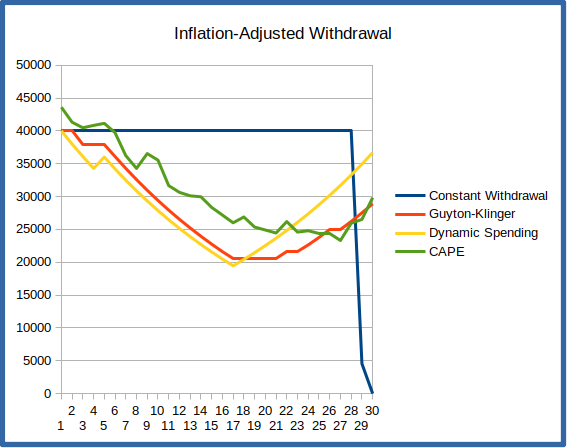
Bad times: Retiring in 1969
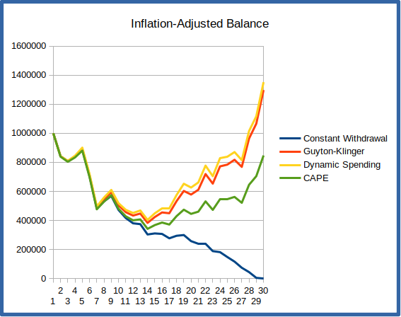
If you had retired in 1969, you’d be in the unfortunate position of encountering the economic doldrums and skyrocketing inflation of the 70’s during your first decade of retirement. This first 10 years is really a crucial period, since poor returns that deplete a significant portion of the portfolio early in retirement can leave a retiree with too low a balance for it to recover when times get good. We see this in the graphs below, which show the annual withdrawals and portfolio balance for the 30-year period starting in 1969.
You can see from the portfolio balance chart that the constant-withdrawal scheme has completely depleted the portfolio by year 29 – you’re broke! The other schemes don’t suffer this fate – they’re specifically designed to cut back on withdrawals when they detect the portfolio is in trouble. The downside is that they consequently leave you with considerably less to live on. Both the Guyton-Klinger and Dynamic Spending approaches have spending down to an inflation-adjusted $20,000 in year 20 (1989), though they do rapidly recover when the market takes off during the 90’s tech boom. The CAPE scheme similarly keeps spending between $25,000 and $35,000 to protect the portfolio. Notice that the CAPE scheme is less reactive than Guyton-Klinger and Dynamic Spending – it neither drops spending as fast when times are tough, nor raises it as quickly when markets recover.
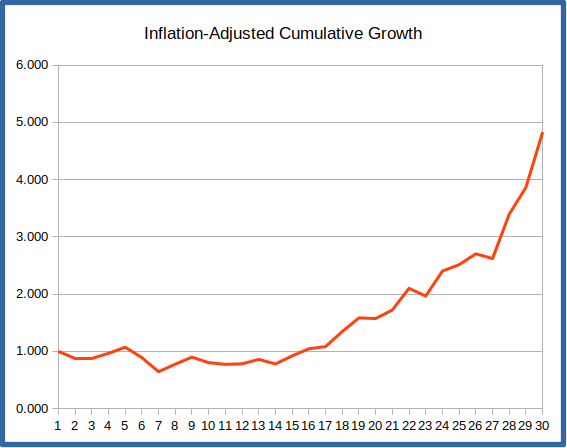
Also shown is the inflation-adjusted cumulative growth rate for investments over this period. This shows what $1 left invested would grow to over time after adjusting for inflation. This chart illustrates the problem – for the first 15 or so years there’s no real growth after inflation. All the withdrawals taken during this period deplete the portfolio without it being able to recover. So even though the latter part of the retirement period covers the huge tech boom of the 90’s, the portfolio may have been mortally wounded before we get to the growth.
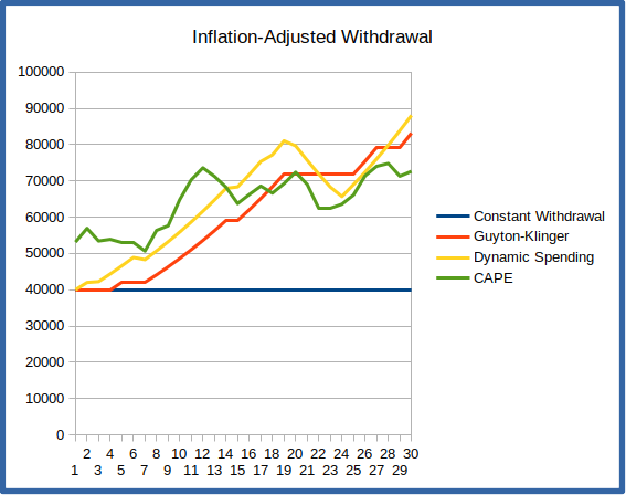
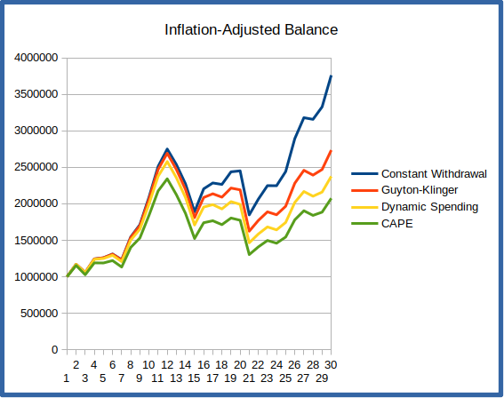
Good times: Retiring in 1989
If you retired in 1989, you’d get the benefit from the tech boom of the 90’s during your first decade of retirement, which would grow your portfolio tremendously even as you took withdrawals. True, you’d eventually run into the tech-bubble burst and even suffer through the market crash in 2008, but the growth of the 90’s would have powered your portfolio to withstand even these blows – a good illustration of how the first decade of retirement is key.
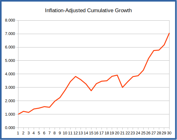
The graphs below illustrate how withdrawals and portfolio balances would change over this period for each of the withdrawal methods. Despite a rapidly growing portfolio, the constant-withdrawal method keeps withdrawals at $40,000 each year, adjusted for inflation. Both the Guyton-Klinger and Dynamic Spending methods steadily increase spending as the portfolio grows, with Dynamic Spending responding a little more quickly. The withdrawal graph shows that the CAPE method starts at a somewhat higher level, but increases a bit more slowly and imposes some drops as market conditions change.
The growth chart helps to explain why life is good in this scenario. Even though growth is pretty much flat and even suffers some significant drops during the second decade of retirement, the strong growth in the first decade has helped to insulate the portfolio from these challenges.
Discussion
The key observation from the above scenarios is that, as expected, the variable-withdrawal strategies react to portfolio balance and/or market conditions to provide a benefit when times are good and belt-tightening when times are bad. The exact behavior differs for the different methods – how much they raise or cut income, and at which points – but they all trend similarly because they’re all focused on the same things.
Conclusion
The above discusses ways to make retirement withdrawal more dependent on things that matter, particularly portfolio performance and economic fundamentals. This might involve tailoring a withdrawal rate to the market conditions at the time of retirement, or adjusting withdrawals throughout retirement. Really, any of these approaches is preferable to choosing a withdrawal rate blindly and sticking to it, which none of us is likely to do anyway. The withdrawal strategies discussed provide some rationale as to what our withdrawals should be, based on conditions at (and throughout) retirement.
A basic question is, “which one is best”? That’s a difficult question to answer because it depends on each retiree’s preferences. Do you want an absolutely rock-steady income year after year, even at the risk of running low on your portfolio? Are you willing to accept ups and downs in income as a means to protect the portfolio value? And if so, how much? The variable spending models discussed here all have parameters that adjust their behavior regarding how significantly and frequently they adjust the withdrawal amount, and finding the right set of parameters to suit one’s tolerance for income changes and portfolio fluctuations is key for each retiree. This is where either a lot of experimentation and research, or consultation with a savvy financial advisor, is essential.
Another article on this website tries to define and quantify some criteria that might be important to a given retiree – things like, which strategy pays out the most on average over all market scenarios (efficiency), and which strategy provides the fewest severe ups and downs in the sequence of annual withdrawals (disruptiveness). The article compares a number of schemes over many market simulations to see how they perform on these criteria. (Spoiler alert: Guyton-Klinger and Dynamic Spending perform very similarly, and well, on these criteria.)
The bottom line is that variable-spending methods are not off-the-shelf ready-to-wear solutions, and these articles just scratch the surface.
Caveat
This information is presented as-is, with no guarantee as to accuracy or freedom from errors. This document and associated spreadsheets are intended as an observation for informational purposes only, and should not be used in retirement planning without cross-checking and correlating with other sources of information and consultation with a certified financial planner. I’m an enthusiast, not a professional, and being human I make mistakes. Your retirement funding is far too important to rely significantly on any unvalidated information!
Worksheet and Simulator Download
- Guyton-Klinger Personal Worksheet (OpenOffice/LibreOffice format)
- Dynamic Spending Personal Worksheet (OpenOffice/LibreOffice format)
- Advanced Market Simulator (OpenOffice/LibreOffice format)
The worksheets and simulator are open-source software licensed under the Gnu General Public License v2. This gives you the right to use these for your purposes, and adapt them (create a derived work) as you see fit as long as you make the new spreadsheet publicly available for other users and include the copyright notice within the spreadsheet. See the link above for license details.
Data source for economic data used in the simulator
Historical returns: Stocks, T.Bonds & T.Bills with premiums, Aswath Damodaran, Stern School of Business, New York University.
References
Is 4% Rule Too High? Rule Inventor Says It Should Be 4.7% Rule, Paul Katzeff, Investors Business Daily, December 22, 2021.
Understanding Sequence Of Return Risk – Safe Withdrawal Rates, Bear Market Crashes, And Bad Decades, Michael Kitces, October 1, 2014.
CAPE Ratio (Shiller PE Ratio): Definition, Formula, Uses, Example, Will Kenton, Investopedia, October 23, 2020.
Resolving the Paradox – Is the Safe Withdrawal Rate
Sometimes Too Safe?, Michael Kitces, May 2008.
Bill Bengen Revisits The 4% Rule Using Shiller’s CAPE Ratio, Michael Kitces’s Research, William Bengen, Financial Advisor Magazine, December 17, 2020.
A rule for all seasons: Vanguard’s dynamic approach to retirement spending, Michael A. DiJoseph, Colleen M. Jaconetti, Zoe B. Odenwalder, and Francis M. Kinniry Jr., Vanguard Research, March 2017.
The Ultimate Guide to Safe Withdrawal Rates – Part 18: Flexibility and the Mechanics of CAPE-Based Rules, Early Retirement Now.
Articles in this series
-
Life Tables and Retirement Planning
-
Retirement Withdrawal Strategies: Guyton-Klinger as a Happy Medium
-
Variable Withdrawal Schemes: Guyton-Klinger, Dynamic Spending, and CAPE-Based
-
Comparing Retirement Withdrawal Schemes: Efficiency, Deficiency, and Disruptiveness
-
Retirement Withdrawal Efficiency Revisited: Variable Lifespan and Annuities
-
Annual or Monthly Withdrawal? Dollar Cost Averaging in Retirement
-
Over-valued, Under-valued, or Just About Right? Assessing Retirement Portfolios in Current Conditions